SlideShare ist ein Scribd-Unternehmen logo
1 von 36
1
3.4 Basic Propagation Mechanisms & Transmission Impairments
(1) Reflection: propagating wave impinges on object with size >> λ
• examples include ground, buildings, walls
(2) Diffraction: transmission path obstructed by objects with edges
• 2nd
ry waves are present throughout space (even behind object)
• gives rise to bending around obstacle (NLOS transmission path)
(3) Scattering propagating wave impinges on object with size < λ
• number of obstacles per unit volume is large (dense)
• examples include rough surfaces, foliage, street signs, lamp posts
2
Models are used to predict received power or path loss (reciprocal)
based on refraction, reflection, scattering
• Large Scale Models
• Fading Models
at high frequencies  diffraction & reflections depend on
• geometry of objects
• EM wave’s, amplitude, phase, & polarization at point of intersection
3
3.5 Reflection: EM wave in 1st
medium impinges on 2nd
medium
• part of the wave is transmitted
• part of the wave is reflected
(1) plane-wave incident on a perfect dielectric (non-conductor)
• part of energy is transmitted (refracted) into 2nd
medium
• part of energy is transmitted (reflected) back into 1st
medium
• assumes no loss of energy from absorption (not practically)
(2) plane-wave incident on a perfect conductor
• all energy is reflected back into the medium
• assumes no loss of energy from absorption (not practically)
4
(3) Γ = Fersnel reflection coefficient relates Electric Field intensity
of reflected & refracted waves to incident wave as a function of:
• material properties,
• polarization of wave
• angle of incidence
• signal frequency
boundary between dielectrics
(reflecting surface)
reflected wave
refracted wave
incident wave
5
(4) Polarization: EM waves are generally polarized
• instantaneous electric field components are in orthogonal
directions
in space represented as either:
(i) sum of 2 spatially orthogonal components (e.g. vertical
& horizontal)
(ii) left-handed or right handed circularly polarized components
• reflected fields from a reflecting surface can be computed using
superposition for any arbitrary polarizationE||
E⊥
6
3.5.1 Reflection from Dielectrics
• assume no loss of energy from absorption
EM wave with E-field incident at ∠θi with boundary between 2
dielectric media
• some energy is reflected into 1st
media at ∠θr
• remaining energy is refracted into 2nd
media at ∠θt
• reflections vary with the polarization of the E-field
plane of incidence
reflecting surface= boundary
between dielectrics
θi
θr
θt
plane of incidence = plane containing incident, reflected, & refracted rays
7
Two distinct cases are used to study arbitrary directions of polarization
(1) Vertical Polarization: (Evi) E-field polarization is
• parallel to the plane of incidence
• normal component to reflecting surface
(2) Horizontal Polarization: (Ehi) E-field polarization is
• perpendicular to the plane of incidence
• parallel component to reflecting surface
plane of incidence
θi
θr
θt
Evi
Ehi
boundary between dielectrics
(reflecting surface)
8
• Ei & Hi = Incident electric and magnetic fields
• Er & Hr = Reflected electric and magnetic fields
• Et = Transmitted (penetrating) electric field
Hi Hr
Ei Er
θi θr
θt
ε1,µ1, σ1
ε2,µ2, σ2
Et
Vertical Polarization: E-field in
the plane of incidence
Hi
HrEi
Er
θi θr
θt
ε1,µ1, σ1
ε2,µ2, σ2
Et
Horizontal Polarization: E-field
normal to plane of incidence
9
(1) EM Parameters of Materials
∀ε = permittivity (dielectric constant): measure of a materials ability
to resist current flow
• µ = permeability: ratio of magnetic induction to magnetic field
intensity
• σ = conductance: ability of a material to conduct electricity,
measured in Ω-1
dielectric constant for perfect dielectric (e.g. perfect reflector of
lossless material) given by
ε0 = 8.85 ×10⁻¹²
F/m
10
often permittivity of a material, ε is related to relative permittivity εr
ε = ε0 εr
lossy dielectric materials will absorb power  permittivity described
with complex dielectric constant
(3.18)where ε’ =
fπ
σ
2
(3.17)ε = ε0 εr -jε’
highly conductive materials 
∀εr & σ are generally insensitive to operating frequency
r
f
εε
σ
0
<
• ε0 and εr are generally constant
• σ may be sensitive to operating frequency
11
Material εr σ σ/εrε0 f (Hz)
Poor Ground 4 0.001 2.82 ×10⁷ 108
Typical Ground 15 0.005 3.77 ×10⁷ 108
Good Ground 25 0.02 9.04 ×10⁷ 108
Sea Water 81 5 6.97 ×10⁹ 108
Fresh Water 81 0.001 1.39 ×10⁶ 108
Brick 4.44 0.001 2.54 ×10⁷
4⋅109
Limestone 7.51 0.028 4.21 ×10⁸
4⋅109
Glass, Corning 707 4 0.00000018 5.08 ×10³ 106
Glass, Corning 707 4 0.000027 7.62 ×10⁵ 108
Glass, Corning 707 4 0.005 1.41 ×10⁸ 1010
12
• because of superposition – only 2 orthogonal polarizations need be
considered to solve general reflection problem
Maxwell’s Equation boundary conditions used to derive (3.19-3.23)
Fresnel reflection coefficients for E-field polarization at reflecting
surface boundary
• Γ|| represents coefficient for || E-field polarization
• Γ⊥ represents coefficient for ⊥ E-field polarization
(2) Reflections, Polarized Components & Fresnel Reflection
Coefficients
13
Fersnel reflection coefficients given by
(i) E-field in plane of incidence (vertical polarization)
Γ|| =
it
it
i
r
E
E
θηθη
θηθη
sinsin
sinsin
12
12
+
−
= (3.19)
(ii) E-field not in plane of incidence (horizontal polarization)
Γ⊥ =
ti
ti
i
r
E
E
θηθη
θηθη
sinsin
sinsin
12
12
+
−
= (3.20)
ηi = intrinsic impedance of the ith
medium
• ratio of electric field to magnetic field for uniform plane wave in
ith
medium
• given by ηi = ii εµ
14
velocity of an EM wave given by ( ) 1−
µε
boundary conditions at surface of incidence obey Snell’s Law
( ) ( ) )90sin()90sin( 222111 θεµθεµ −=− (3.21)
θi = θr (3.22)
Er = Γ Ei (3.23a)
Et = (1 + Γ )Ei (3.23b)
Γ is either Γ|| or Γ⊥ depending on polarization
• | Γ | ≈ 1  for a perfect conductor, wave is fully reflected
• | Γ | ≈ 0  for a lossy material, wave is fully refracted








−−= −
)90sin(sin90
2
11
it θ
η
η
θ
15
• radio wave propagating in free space (1st
medium is free space)
• µ1 = µ2
Γ|| =
irir
irir
θεθε
θεθε
2
2
cossin
cossin
−+
−+−
(3.24)
Γ⊥ =
iri
iri
θεθ
θεθ
2
2
cossin
cossin
−+
−−
(3.25)
Simplification of reflection coefficients for vertical and horizontal
polarization assuming:
Elliptically Polarized Waves have both vertical & horizontal components
• waves can be depolarized (broken down) into vertical & horizontal
E-field components
• superposition can be used to determine transmitted & reflected
waves
16
(3) General Case of reflection or transmission
• horizontal & vertical axes of spatial coordinates may not coincide
with || & ⊥ axes of propagating waves
• for wave propagating out of the page  define angle ∠θ
measured counter clock-wise from horizontal axes
spatial horizontal axis
spatial vertical axis
θ
⊥
||
orthogonal components
of propagating wave
17
↔vertical & horizontal
polarized components
components perpendicular
& parallel to plane of incidence
Ei
H , Ei
V Ed
H , Ed
V
• Ed
H , Ed
V = depolarized field components along the horizontal &
vertical axes
• Ei
H , Ei
V = horizontal & vertical polarized components of incident
wave
relationship of vertical & horizontal field components at the dielectric
boundary
Ed
H, Ed
V Ei
H , Ei
V = Time Varying Components of E-field






=





i
v
i
H
C
T
d
v
d
H
E
E
RDR
E
E
(3.26)
- E-field components may be represented by phasors
18
for case of reflection:
• D⊥⊥ = Γ⊥
• D|| || = Γ||
for case of refraction (transmission):
• D⊥⊥ = 1+ Γ⊥
• D|| || = 1+ Γ||
R = 





− θθ
θθ
cossin
sincos
, θ = angle between two sets of axes
DC = 




 ⊥⊥
||||0
0
D
D
R = transformation matrix that maps E-field components
DC = depolarization matrix
19
1.0
0.8
0.6
0.4
0.2
0.0
0 10 20 30 40 50 60 70 80 90
|Γ|||
εr=12
εr=4
angle of incidence (θi)
Brewster Angle (θB)
for εr=12
vertical polarization
(E-field in plane of incidence)
for θi < θB: a larger dielectric constant  smaller Γ|| & smaller Er
for θi > θB: a larger dielectric constant  larger Γ|| & larger Er
Plot of Reflection Coefficients for Parallel Polarization for εr= 12, 4
20
εr=12
εr=4
|Γ⊥|1.0
0.9
0.8
0.7
0.6
0.5
0.4
0.3
0 10 20 30 40 50 60 70 80 90
angle of incidence (θi)
horizontal polarization
(E-field not in plane of
incidence)
for given θi: larger dielectric constant  larger Γ⊥ and larger Er
Plot of Reflection Coefficients for Perpendicular Polarization for εr=
12, 4
21
e.g. let medium 1 = free space & medium 2 = dielectric
• if θi  0o
(wave is parallel to ground)
• then independent of εr, coefficients |Γ⊥|  1 and |Γ|||  1
Γ|| = 1
cos
cos
cossin
cossin
2
2
0
2
2
=
−
−
=
−+
−+−
= ir
ir
irir
irir
i
θε
θε
θεθε
θεθε
θ
Γ⊥ = 1
cos
cos
cossin
cossin
2
2
0
2
2
−=
−
−−
=
−+
−−
= ir
ir
iri
iri
i
θε
θε
θεθ
θεθ
θ
thus, if incident wave grazes the earth
• ground may be modeled as a perfect reflector with |Γ| = 1
• regardless of polarization or ground dielectric properties
• horizontal polarization results in 180° phase shift
22
3.5.2 Brewster Angle = θB
• Brewster angle only occurs for vertical (parallel) polarization
• angle at which no reflection occurs in medium of origin
• occurs when incident angle θi is such that Γ|| = 0  θi = θB
• if 1st
medium = free space & 2nd
medium has relative permittivity εr
then (3.27) can be expressed as
1
1
2
−
−
r
r
ε
ε
sin(θB) = (3.28
)
sin(θB) =
21
1
εε
ε
+
(3.27
)
θB satisfies
23
e.g. 1st
medium = free space
Let εr = 4 
116
14
−
−
sin(θB) = = 0.44
θB = sin-1
(0.44) = 26.6o
Let εr = 15 
115
115
2
−
−
sin(θB) = = 0.25
θB = sin-1
(0.25) = 14.5o
24
3.6 Ground Reflection – 2 Ray Model
Free Space Propagation model is inaccurate for most mobile RF
channels
2 Ray Ground Reflection model considers both LOS path & ground
reflected path
• based on geometric optics
• reasonably accurate for predicting large scale signal strength for
distances of several km
• useful for
- mobile RF systems which use tall towers (> 50m)
- LOS microcell channels in urban environments
Assume
• maximum LOS distances d ≈ 10km
• earth is flat
25
Let E0 = free space E-field (V/m) at distance d0
• Propagating Free Space E-field at distance d > d0 is given by
E(d,t) = 











−
c
d
tw
d
dE
ccos00
(3.33)
• E-field’s envelope at distance d from transmitter given by
|E(d,t)| = E0 d0/d
(1) Determine Total Received E-field (in V/m) ETOT
ELOS
Ei
Er
= Eg
θi θ0
d
ETOT is combination of ELOS & Eg
• ELOS = E-field of LOS component
• Eg = E-field of ground reflected component
• θi = θr
26
d’
d”
ELOS
Ei
Egθi θ0
d
ht
hr
E-field for LOS and reflected wave relative to E0 given by:
and ETOT = ELOS + Eg
ELOS(d’,t) = 











−
c
d
tw
d
dE
c
'
cos
'
00
(3.34)
Eg(d”,t) = 











−
c
d
tw
d
dE
Γ c
"
cos
"
00
(3.35)
assumes LOS & reflected waves arrive at the receiver with
- d’ = distance of LOS wave
- d” = distance of reflected wave
27
From laws of reflection in dielectrics (section 3.5.1)
θi = θ0 (3.36)
Eg = Γ Ei (3.37a)
Et = (1+Γ) Ei (3.37b)
Γ = reflection coefficient for ground
Eg
d’
d”
ELOS
Ei
θi θ0
Et
28
resultant E-field is vector sum of ELOS and Eg
• total E-field Envelope is given by |ETOT| = |ELOS + Eg| (3.38)
• total electric field given by
+











−
c
d
tw
d
dE
c
'
cos
'
00












−−
c
d
tw
d
dE
c
"
cos
"
)1( 00
(3.39)ETOT(d,t) =
Assume
i. perfect horizontal E-field Polarization
ii. perfect ground reflection
iii. small θi (grazing incidence)  Γ ≈ -1 & Et ≈ 0
• reflected wave & incident wave have equal magnitude
• reflected wave is 180o
out of phase with incident wave
• transmitted wave ≈ 0
29
• path difference ∆ = d” – d’ determined from method of images
( ) ( ) 2222
dhhdhh rtrt +−−++∆ = (3-40)
if d >> hr + ht  Taylor series approximations yields (from 3-40)
∆ ≈
d
hh rt2 (3-41)
(2) Compute Phase Difference & Delay Between Two Components
ELOS
d
d’
d”θi θ0
ht
hr
∆h
ht+hr
Ei Eg
30
once ∆ is known  we can compute
• phase difference θ∆ =
c
wc⋅∆
=
∆
λ
π2
(3-42)
• time delay τd =
cfc π
θ
2
∆
=
∆
(3-43)
As d becomes large  ∆ = d”-d’ becomes small
• amplitudes of ELOS & Eg are nearly identical & differ only in phase
"'
000000
d
dE
d
dE
d
dE
≈≈ (3.44)
if Δ = λ/n  θ∆ = 2π/n0 π 2π
λ
Δ
31
(3) Evaluate E-field when reflected path arrives at receiver
( )0cos
"
)1(
'"
cos
'
0000
d
dE
c
dd
w
d
dE
c −+










 −
(3.45)ETOT(d,t)|t=d”/c =
t = d”/creflected path arrives at receiver at






−




 ∆
1cos00
c
w
d
dE
c≈
( )[ ]1cos00
−∆θ
d
dE
=
( )[ ]100
−∠ ∆θ
d
dE
=
32
(3.46)
( )( )∆∆ +−





θθ 22
2
00
sin1cos
d
dE
=( ) ∆∆ 





+−





θθ 2
2
002
2
00
1 sin
d
dE
cos
d
dE
|ETOT(d)|=
=
=











 ∆
2
sin2 00 θ
d
dE
∆−





θcos2200
d
dE
(3.47)
(3.48)
ETOT
"
00
d
dE
'd
dE 00
θ∆
Use phasor diagram to find resultant E-field from combined direct &
ground reflected rays:
(4) Determine exact E-field for 2-ray ground model at distance d
33
As d increases  ETOT(d) decreases in oscillatory manner
• local maxima 6dB > free space value
• local minima ≈ -∞ dB (cancellation)
• once d is large enough  θΔ < π & ETOT(d) falls off asymtotically
with increasing d
-50
-60
-70
-80
-90
-100
-110
-120
-130
-140
101
102
103
104
m
fc = 3GHz
fc = 7GHz
fc = 11GHz
Propagation Loss ht = hr = 1, Gt = Gr = 0dB
34
if d satisfies 3.50  total E-field can be approximated as:
k is a constant related to E0 ht,hr, and λ
rad
d
hh rt
3.0
22
2
1
2
<≈
∆
=∆
λ
π
λ
πθ
(3.49)
d > (3.50)
λλ
π rtrt hhhh 20
3
20
≈this implies
For phase difference, θ∆ < 0.6 radians (34o
) sin(0.5θ∆ ) ≈ θ∆











 ∆
2
2 00 θ
d
dE
|ETOT(d)| ≈
e.g. at 900MHz  if ∆ < 0.03m  total E-field decays with d2
2
00 22
d
k
d
hh
d
dE rt
≈





λ
π
(3.51)ETOT(d) ≈ V/m
35
Received Power at d is related to square of E-field by 3.2, 3.15, & 3.51
Pr(d) = (3.52b)





=
π
λ
ππ 4120
)(
120
)( 222
0 rR
e
GdE
A
dE
Pr(d) = 4
22
d
hh
GGP rt
rtt (3.52a)
• received power falls off at 40dB/decade
• receive power & path loss become independent of frequency
rthhif d >>
36
Path Loss for 2-ray model with antenna gains is expressed as:
• for short Tx-Rx distances use (3.39) to compute total E field
• evaluate (3.42) for θ∆ = π (180o
)  d = 4hthr/λ is where the ground
appears in 1st
Fresnel Zone between Tx & Rx
- 1st
Fresnel distance zone is useful parameter in microcell path
loss models
PL(dB) = 40log d - (10logGt + 10logGr + 20log ht + 20 log hr ) (3.53)
PL =
1
4
22 −






=
d
hh
GG
P
P rt
rt
r
t
• 3.50 must hold

Weitere ähnliche Inhalte

Was ist angesagt? (20)

Linear Antenna
Linear AntennaLinear Antenna
Linear Antenna
 
Radar
RadarRadar
Radar
 
Radar Basics
Radar BasicsRadar Basics
Radar Basics
 
Wave guide tees
Wave guide teesWave guide tees
Wave guide tees
 
Cw and fm cw radar
Cw and fm cw radarCw and fm cw radar
Cw and fm cw radar
 
Satellite link design
Satellite link designSatellite link design
Satellite link design
 
Radar fundamentals
Radar fundamentalsRadar fundamentals
Radar fundamentals
 
Frequency bands
Frequency bandsFrequency bands
Frequency bands
 
microwave-engineering
microwave-engineeringmicrowave-engineering
microwave-engineering
 
Radar 2009 a 11 waveforms and pulse compression
Radar 2009 a 11 waveforms and pulse compressionRadar 2009 a 11 waveforms and pulse compression
Radar 2009 a 11 waveforms and pulse compression
 
Antenna PARAMETERS
Antenna PARAMETERSAntenna PARAMETERS
Antenna PARAMETERS
 
Spread Spectrum System
Spread Spectrum SystemSpread Spectrum System
Spread Spectrum System
 
array and phased array antennna
array and phased array antennnaarray and phased array antennna
array and phased array antennna
 
Satellite communication Basics
Satellite communication BasicsSatellite communication Basics
Satellite communication Basics
 
Software Defined Radio (SDR)
Software Defined Radio (SDR)Software Defined Radio (SDR)
Software Defined Radio (SDR)
 
radar technology
radar technologyradar technology
radar technology
 
Ultra wide band technology
Ultra wide band technology Ultra wide band technology
Ultra wide band technology
 
Study of Radar System PPT
Study of Radar System PPTStudy of Radar System PPT
Study of Radar System PPT
 
Radar 2009 a 4 radar equation
Radar 2009 a  4 radar equationRadar 2009 a  4 radar equation
Radar 2009 a 4 radar equation
 
Radar system
Radar systemRadar system
Radar system
 

Ähnlich wie Wave propagation properties

Unit V-Electromagnetic Fields-Normal incidence at a plane dielectric boundary...
Unit V-Electromagnetic Fields-Normal incidence at a plane dielectric boundary...Unit V-Electromagnetic Fields-Normal incidence at a plane dielectric boundary...
Unit V-Electromagnetic Fields-Normal incidence at a plane dielectric boundary...Dr.SHANTHI K.G
 
Numerical studies of the radiation patterns of resistively loaded dipoles
Numerical studies of the radiation patterns of resistively loaded dipolesNumerical studies of the radiation patterns of resistively loaded dipoles
Numerical studies of the radiation patterns of resistively loaded dipolesLeonid Krinitsky
 
The Influence Of Infinite Impedance Flanges On The Electromagnetic Field Of A...
The Influence Of Infinite Impedance Flanges On The Electromagnetic Field Of A...The Influence Of Infinite Impedance Flanges On The Electromagnetic Field Of A...
The Influence Of Infinite Impedance Flanges On The Electromagnetic Field Of A...IJERA Editor
 
AntBrief123A12-6-07.pptMaxwell’s Equations & EM Waves
AntBrief123A12-6-07.pptMaxwell’s Equations & EM WavesAntBrief123A12-6-07.pptMaxwell’s Equations & EM Waves
AntBrief123A12-6-07.pptMaxwell’s Equations & EM Wavesvasuhisrinivasan
 
12330707_0ad850b3-72c9-43d9-9690-b0f996c54dd3.pdf
12330707_0ad850b3-72c9-43d9-9690-b0f996c54dd3.pdf12330707_0ad850b3-72c9-43d9-9690-b0f996c54dd3.pdf
12330707_0ad850b3-72c9-43d9-9690-b0f996c54dd3.pdfsayanduttaclass10bro
 
Em theory lecture
Em theory lectureEm theory lecture
Em theory lecturej sarma
 
Class 12th Physics wave optics ppt part 2
Class 12th Physics wave optics ppt part 2 Class 12th Physics wave optics ppt part 2
Class 12th Physics wave optics ppt part 2 Arpit Meena
 
EC6602 - AWP UNIT3
EC6602 - AWP UNIT3EC6602 - AWP UNIT3
EC6602 - AWP UNIT3krishnamrm
 
Wave Optics Class 12 Part-2
Wave Optics Class 12 Part-2Wave Optics Class 12 Part-2
Wave Optics Class 12 Part-2Self-employed
 
Large scale path loss 1
Large scale path loss 1Large scale path loss 1
Large scale path loss 1Vrince Vimal
 

Ähnlich wie Wave propagation properties (20)

5 slides
5 slides5 slides
5 slides
 
Unit V-Electromagnetic Fields-Normal incidence at a plane dielectric boundary...
Unit V-Electromagnetic Fields-Normal incidence at a plane dielectric boundary...Unit V-Electromagnetic Fields-Normal incidence at a plane dielectric boundary...
Unit V-Electromagnetic Fields-Normal incidence at a plane dielectric boundary...
 
Lecture15_Hall_effect.pdf
Lecture15_Hall_effect.pdfLecture15_Hall_effect.pdf
Lecture15_Hall_effect.pdf
 
Numerical studies of the radiation patterns of resistively loaded dipoles
Numerical studies of the radiation patterns of resistively loaded dipolesNumerical studies of the radiation patterns of resistively loaded dipoles
Numerical studies of the radiation patterns of resistively loaded dipoles
 
Emt
EmtEmt
Emt
 
Q50202104110
Q50202104110Q50202104110
Q50202104110
 
Q50202104110
Q50202104110Q50202104110
Q50202104110
 
Q50202104110
Q50202104110Q50202104110
Q50202104110
 
Q50202104110
Q50202104110Q50202104110
Q50202104110
 
Q50202104110
Q50202104110Q50202104110
Q50202104110
 
The Influence Of Infinite Impedance Flanges On The Electromagnetic Field Of A...
The Influence Of Infinite Impedance Flanges On The Electromagnetic Field Of A...The Influence Of Infinite Impedance Flanges On The Electromagnetic Field Of A...
The Influence Of Infinite Impedance Flanges On The Electromagnetic Field Of A...
 
AntBrief123A12-6-07.pptMaxwell’s Equations & EM Waves
AntBrief123A12-6-07.pptMaxwell’s Equations & EM WavesAntBrief123A12-6-07.pptMaxwell’s Equations & EM Waves
AntBrief123A12-6-07.pptMaxwell’s Equations & EM Waves
 
12330707_0ad850b3-72c9-43d9-9690-b0f996c54dd3.pdf
12330707_0ad850b3-72c9-43d9-9690-b0f996c54dd3.pdf12330707_0ad850b3-72c9-43d9-9690-b0f996c54dd3.pdf
12330707_0ad850b3-72c9-43d9-9690-b0f996c54dd3.pdf
 
Electro magnetic waves
Electro magnetic wavesElectro magnetic waves
Electro magnetic waves
 
Em theory lecture
Em theory lectureEm theory lecture
Em theory lecture
 
Class 12th Physics wave optics ppt part 2
Class 12th Physics wave optics ppt part 2 Class 12th Physics wave optics ppt part 2
Class 12th Physics wave optics ppt part 2
 
EC6602 - AWP UNIT3
EC6602 - AWP UNIT3EC6602 - AWP UNIT3
EC6602 - AWP UNIT3
 
Wave Optics Class 12 Part-2
Wave Optics Class 12 Part-2Wave Optics Class 12 Part-2
Wave Optics Class 12 Part-2
 
Large scale path loss 1
Large scale path loss 1Large scale path loss 1
Large scale path loss 1
 
4_wave_optics_2.ppt
4_wave_optics_2.ppt4_wave_optics_2.ppt
4_wave_optics_2.ppt
 

Mehr von Izah Asmadi

Aircraft Communication Topic 10 instrument landing systems
Aircraft Communication Topic 10 instrument landing systemsAircraft Communication Topic 10 instrument landing systems
Aircraft Communication Topic 10 instrument landing systemsIzah Asmadi
 
Aircraft Communication Topic 9 vhf omni range (vor)
Aircraft Communication  Topic 9 vhf omni range (vor)Aircraft Communication  Topic 9 vhf omni range (vor)
Aircraft Communication Topic 9 vhf omni range (vor)Izah Asmadi
 
Aircraft Communication Topic 8 automatic direction finder
Aircraft Communication  Topic 8 automatic direction finderAircraft Communication  Topic 8 automatic direction finder
Aircraft Communication Topic 8 automatic direction finderIzah Asmadi
 
Aircraft Communication Topic 7 elt, cvr and fdr
Aircraft Communication  Topic 7 elt, cvr and fdrAircraft Communication  Topic 7 elt, cvr and fdr
Aircraft Communication Topic 7 elt, cvr and fdrIzah Asmadi
 
Aircraft Communication Topic 6 pa system
Aircraft Communication  Topic 6 pa systemAircraft Communication  Topic 6 pa system
Aircraft Communication Topic 6 pa systemIzah Asmadi
 
Aircraft Communication Topic 5 selcal and data link system
Aircraft Communication  Topic 5 selcal and data link systemAircraft Communication  Topic 5 selcal and data link system
Aircraft Communication Topic 5 selcal and data link systemIzah Asmadi
 
Aircraft Communication Topic 4 vhf communication system
Aircraft Communication  Topic 4 vhf communication systemAircraft Communication  Topic 4 vhf communication system
Aircraft Communication Topic 4 vhf communication systemIzah Asmadi
 
Aircraft Communication Topic 4 hf communication system
Aircraft Communication  Topic 4 hf communication systemAircraft Communication  Topic 4 hf communication system
Aircraft Communication Topic 4 hf communication systemIzah Asmadi
 
Aircraft Communication Topic 2 modulation and propagation of radio waves
Aircraft Communication  Topic 2 modulation and propagation of radio wavesAircraft Communication  Topic 2 modulation and propagation of radio waves
Aircraft Communication Topic 2 modulation and propagation of radio wavesIzah Asmadi
 
Topic 1 basic radio wave properties
Topic 1 basic radio wave propertiesTopic 1 basic radio wave properties
Topic 1 basic radio wave propertiesIzah Asmadi
 
Aircraft Communication Topic 3 radio components
Aircraft Communication  Topic 3 radio componentsAircraft Communication  Topic 3 radio components
Aircraft Communication Topic 3 radio componentsIzah Asmadi
 
Business ethics C8 -ethics_technology
Business ethics C8  -ethics_technologyBusiness ethics C8  -ethics_technology
Business ethics C8 -ethics_technologyIzah Asmadi
 
Business ethics C7 -business_ethics_environmental_issues
Business ethics C7  -business_ethics_environmental_issuesBusiness ethics C7  -business_ethics_environmental_issues
Business ethics C7 -business_ethics_environmental_issuesIzah Asmadi
 
C6 -ethics_and_government_compatibility_mode_
C6  -ethics_and_government_compatibility_mode_C6  -ethics_and_government_compatibility_mode_
C6 -ethics_and_government_compatibility_mode_Izah Asmadi
 
Business ethics C5 -organizational_ethics_compatibility_mode_
Business ethics C5  -organizational_ethics_compatibility_mode_Business ethics C5  -organizational_ethics_compatibility_mode_
Business ethics C5 -organizational_ethics_compatibility_mode_Izah Asmadi
 
Business ethics C4 -corporate_social_responsibility_compatibility_mode_
Business ethics C4  -corporate_social_responsibility_compatibility_mode_Business ethics C4  -corporate_social_responsibility_compatibility_mode_
Business ethics C4 -corporate_social_responsibility_compatibility_mode_Izah Asmadi
 
Business ethics C3 theories principles in_business_ethics
Business ethics C3 theories principles in_business_ethicsBusiness ethics C3 theories principles in_business_ethics
Business ethics C3 theories principles in_business_ethicsIzah Asmadi
 
Business ethics C1 -moral_ethics_ethical_dilemma
Business ethics C1  -moral_ethics_ethical_dilemmaBusiness ethics C1  -moral_ethics_ethical_dilemma
Business ethics C1 -moral_ethics_ethical_dilemmaIzah Asmadi
 
Business ethics C2 -business_and_society
Business ethics C2  -business_and_societyBusiness ethics C2  -business_and_society
Business ethics C2 -business_and_societyIzah Asmadi
 
Project Management Ch11 Project Scheduling Critical Chain
Project Management Ch11 Project Scheduling Critical ChainProject Management Ch11 Project Scheduling Critical Chain
Project Management Ch11 Project Scheduling Critical ChainIzah Asmadi
 

Mehr von Izah Asmadi (20)

Aircraft Communication Topic 10 instrument landing systems
Aircraft Communication Topic 10 instrument landing systemsAircraft Communication Topic 10 instrument landing systems
Aircraft Communication Topic 10 instrument landing systems
 
Aircraft Communication Topic 9 vhf omni range (vor)
Aircraft Communication  Topic 9 vhf omni range (vor)Aircraft Communication  Topic 9 vhf omni range (vor)
Aircraft Communication Topic 9 vhf omni range (vor)
 
Aircraft Communication Topic 8 automatic direction finder
Aircraft Communication  Topic 8 automatic direction finderAircraft Communication  Topic 8 automatic direction finder
Aircraft Communication Topic 8 automatic direction finder
 
Aircraft Communication Topic 7 elt, cvr and fdr
Aircraft Communication  Topic 7 elt, cvr and fdrAircraft Communication  Topic 7 elt, cvr and fdr
Aircraft Communication Topic 7 elt, cvr and fdr
 
Aircraft Communication Topic 6 pa system
Aircraft Communication  Topic 6 pa systemAircraft Communication  Topic 6 pa system
Aircraft Communication Topic 6 pa system
 
Aircraft Communication Topic 5 selcal and data link system
Aircraft Communication  Topic 5 selcal and data link systemAircraft Communication  Topic 5 selcal and data link system
Aircraft Communication Topic 5 selcal and data link system
 
Aircraft Communication Topic 4 vhf communication system
Aircraft Communication  Topic 4 vhf communication systemAircraft Communication  Topic 4 vhf communication system
Aircraft Communication Topic 4 vhf communication system
 
Aircraft Communication Topic 4 hf communication system
Aircraft Communication  Topic 4 hf communication systemAircraft Communication  Topic 4 hf communication system
Aircraft Communication Topic 4 hf communication system
 
Aircraft Communication Topic 2 modulation and propagation of radio waves
Aircraft Communication  Topic 2 modulation and propagation of radio wavesAircraft Communication  Topic 2 modulation and propagation of radio waves
Aircraft Communication Topic 2 modulation and propagation of radio waves
 
Topic 1 basic radio wave properties
Topic 1 basic radio wave propertiesTopic 1 basic radio wave properties
Topic 1 basic radio wave properties
 
Aircraft Communication Topic 3 radio components
Aircraft Communication  Topic 3 radio componentsAircraft Communication  Topic 3 radio components
Aircraft Communication Topic 3 radio components
 
Business ethics C8 -ethics_technology
Business ethics C8  -ethics_technologyBusiness ethics C8  -ethics_technology
Business ethics C8 -ethics_technology
 
Business ethics C7 -business_ethics_environmental_issues
Business ethics C7  -business_ethics_environmental_issuesBusiness ethics C7  -business_ethics_environmental_issues
Business ethics C7 -business_ethics_environmental_issues
 
C6 -ethics_and_government_compatibility_mode_
C6  -ethics_and_government_compatibility_mode_C6  -ethics_and_government_compatibility_mode_
C6 -ethics_and_government_compatibility_mode_
 
Business ethics C5 -organizational_ethics_compatibility_mode_
Business ethics C5  -organizational_ethics_compatibility_mode_Business ethics C5  -organizational_ethics_compatibility_mode_
Business ethics C5 -organizational_ethics_compatibility_mode_
 
Business ethics C4 -corporate_social_responsibility_compatibility_mode_
Business ethics C4  -corporate_social_responsibility_compatibility_mode_Business ethics C4  -corporate_social_responsibility_compatibility_mode_
Business ethics C4 -corporate_social_responsibility_compatibility_mode_
 
Business ethics C3 theories principles in_business_ethics
Business ethics C3 theories principles in_business_ethicsBusiness ethics C3 theories principles in_business_ethics
Business ethics C3 theories principles in_business_ethics
 
Business ethics C1 -moral_ethics_ethical_dilemma
Business ethics C1  -moral_ethics_ethical_dilemmaBusiness ethics C1  -moral_ethics_ethical_dilemma
Business ethics C1 -moral_ethics_ethical_dilemma
 
Business ethics C2 -business_and_society
Business ethics C2  -business_and_societyBusiness ethics C2  -business_and_society
Business ethics C2 -business_and_society
 
Project Management Ch11 Project Scheduling Critical Chain
Project Management Ch11 Project Scheduling Critical ChainProject Management Ch11 Project Scheduling Critical Chain
Project Management Ch11 Project Scheduling Critical Chain
 

Kürzlich hochgeladen

SAP Build Work Zone - Overview L2-L3.pptx
SAP Build Work Zone - Overview L2-L3.pptxSAP Build Work Zone - Overview L2-L3.pptx
SAP Build Work Zone - Overview L2-L3.pptxNavinnSomaal
 
Unraveling Multimodality with Large Language Models.pdf
Unraveling Multimodality with Large Language Models.pdfUnraveling Multimodality with Large Language Models.pdf
Unraveling Multimodality with Large Language Models.pdfAlex Barbosa Coqueiro
 
Advanced Test Driven-Development @ php[tek] 2024
Advanced Test Driven-Development @ php[tek] 2024Advanced Test Driven-Development @ php[tek] 2024
Advanced Test Driven-Development @ php[tek] 2024Scott Keck-Warren
 
H2O.ai CEO/Founder: Sri Ambati Keynote at Wells Fargo Day
H2O.ai CEO/Founder: Sri Ambati Keynote at Wells Fargo DayH2O.ai CEO/Founder: Sri Ambati Keynote at Wells Fargo Day
H2O.ai CEO/Founder: Sri Ambati Keynote at Wells Fargo DaySri Ambati
 
How to write a Business Continuity Plan
How to write a Business Continuity PlanHow to write a Business Continuity Plan
How to write a Business Continuity PlanDatabarracks
 
Connect Wave/ connectwave Pitch Deck Presentation
Connect Wave/ connectwave Pitch Deck PresentationConnect Wave/ connectwave Pitch Deck Presentation
Connect Wave/ connectwave Pitch Deck PresentationSlibray Presentation
 
"Debugging python applications inside k8s environment", Andrii Soldatenko
"Debugging python applications inside k8s environment", Andrii Soldatenko"Debugging python applications inside k8s environment", Andrii Soldatenko
"Debugging python applications inside k8s environment", Andrii SoldatenkoFwdays
 
"ML in Production",Oleksandr Bagan
"ML in Production",Oleksandr Bagan"ML in Production",Oleksandr Bagan
"ML in Production",Oleksandr BaganFwdays
 
New from BookNet Canada for 2024: BNC CataList - Tech Forum 2024
New from BookNet Canada for 2024: BNC CataList - Tech Forum 2024New from BookNet Canada for 2024: BNC CataList - Tech Forum 2024
New from BookNet Canada for 2024: BNC CataList - Tech Forum 2024BookNet Canada
 
Take control of your SAP testing with UiPath Test Suite
Take control of your SAP testing with UiPath Test SuiteTake control of your SAP testing with UiPath Test Suite
Take control of your SAP testing with UiPath Test SuiteDianaGray10
 
DSPy a system for AI to Write Prompts and Do Fine Tuning
DSPy a system for AI to Write Prompts and Do Fine TuningDSPy a system for AI to Write Prompts and Do Fine Tuning
DSPy a system for AI to Write Prompts and Do Fine TuningLars Bell
 
Tampa BSides - Chef's Tour of Microsoft Security Adoption Framework (SAF)
Tampa BSides - Chef's Tour of Microsoft Security Adoption Framework (SAF)Tampa BSides - Chef's Tour of Microsoft Security Adoption Framework (SAF)
Tampa BSides - Chef's Tour of Microsoft Security Adoption Framework (SAF)Mark Simos
 
Ensuring Technical Readiness For Copilot in Microsoft 365
Ensuring Technical Readiness For Copilot in Microsoft 365Ensuring Technical Readiness For Copilot in Microsoft 365
Ensuring Technical Readiness For Copilot in Microsoft 3652toLead Limited
 
CloudStudio User manual (basic edition):
CloudStudio User manual (basic edition):CloudStudio User manual (basic edition):
CloudStudio User manual (basic edition):comworks
 
Are Multi-Cloud and Serverless Good or Bad?
Are Multi-Cloud and Serverless Good or Bad?Are Multi-Cloud and Serverless Good or Bad?
Are Multi-Cloud and Serverless Good or Bad?Mattias Andersson
 
Streamlining Python Development: A Guide to a Modern Project Setup
Streamlining Python Development: A Guide to a Modern Project SetupStreamlining Python Development: A Guide to a Modern Project Setup
Streamlining Python Development: A Guide to a Modern Project SetupFlorian Wilhelm
 
Hyperautomation and AI/ML: A Strategy for Digital Transformation Success.pdf
Hyperautomation and AI/ML: A Strategy for Digital Transformation Success.pdfHyperautomation and AI/ML: A Strategy for Digital Transformation Success.pdf
Hyperautomation and AI/ML: A Strategy for Digital Transformation Success.pdfPrecisely
 
TrustArc Webinar - How to Build Consumer Trust Through Data Privacy
TrustArc Webinar - How to Build Consumer Trust Through Data PrivacyTrustArc Webinar - How to Build Consumer Trust Through Data Privacy
TrustArc Webinar - How to Build Consumer Trust Through Data PrivacyTrustArc
 
Dev Dives: Streamline document processing with UiPath Studio Web
Dev Dives: Streamline document processing with UiPath Studio WebDev Dives: Streamline document processing with UiPath Studio Web
Dev Dives: Streamline document processing with UiPath Studio WebUiPathCommunity
 

Kürzlich hochgeladen (20)

SAP Build Work Zone - Overview L2-L3.pptx
SAP Build Work Zone - Overview L2-L3.pptxSAP Build Work Zone - Overview L2-L3.pptx
SAP Build Work Zone - Overview L2-L3.pptx
 
Unraveling Multimodality with Large Language Models.pdf
Unraveling Multimodality with Large Language Models.pdfUnraveling Multimodality with Large Language Models.pdf
Unraveling Multimodality with Large Language Models.pdf
 
Advanced Test Driven-Development @ php[tek] 2024
Advanced Test Driven-Development @ php[tek] 2024Advanced Test Driven-Development @ php[tek] 2024
Advanced Test Driven-Development @ php[tek] 2024
 
H2O.ai CEO/Founder: Sri Ambati Keynote at Wells Fargo Day
H2O.ai CEO/Founder: Sri Ambati Keynote at Wells Fargo DayH2O.ai CEO/Founder: Sri Ambati Keynote at Wells Fargo Day
H2O.ai CEO/Founder: Sri Ambati Keynote at Wells Fargo Day
 
How to write a Business Continuity Plan
How to write a Business Continuity PlanHow to write a Business Continuity Plan
How to write a Business Continuity Plan
 
Connect Wave/ connectwave Pitch Deck Presentation
Connect Wave/ connectwave Pitch Deck PresentationConnect Wave/ connectwave Pitch Deck Presentation
Connect Wave/ connectwave Pitch Deck Presentation
 
"Debugging python applications inside k8s environment", Andrii Soldatenko
"Debugging python applications inside k8s environment", Andrii Soldatenko"Debugging python applications inside k8s environment", Andrii Soldatenko
"Debugging python applications inside k8s environment", Andrii Soldatenko
 
"ML in Production",Oleksandr Bagan
"ML in Production",Oleksandr Bagan"ML in Production",Oleksandr Bagan
"ML in Production",Oleksandr Bagan
 
New from BookNet Canada for 2024: BNC CataList - Tech Forum 2024
New from BookNet Canada for 2024: BNC CataList - Tech Forum 2024New from BookNet Canada for 2024: BNC CataList - Tech Forum 2024
New from BookNet Canada for 2024: BNC CataList - Tech Forum 2024
 
Take control of your SAP testing with UiPath Test Suite
Take control of your SAP testing with UiPath Test SuiteTake control of your SAP testing with UiPath Test Suite
Take control of your SAP testing with UiPath Test Suite
 
DSPy a system for AI to Write Prompts and Do Fine Tuning
DSPy a system for AI to Write Prompts and Do Fine TuningDSPy a system for AI to Write Prompts and Do Fine Tuning
DSPy a system for AI to Write Prompts and Do Fine Tuning
 
Tampa BSides - Chef's Tour of Microsoft Security Adoption Framework (SAF)
Tampa BSides - Chef's Tour of Microsoft Security Adoption Framework (SAF)Tampa BSides - Chef's Tour of Microsoft Security Adoption Framework (SAF)
Tampa BSides - Chef's Tour of Microsoft Security Adoption Framework (SAF)
 
Ensuring Technical Readiness For Copilot in Microsoft 365
Ensuring Technical Readiness For Copilot in Microsoft 365Ensuring Technical Readiness For Copilot in Microsoft 365
Ensuring Technical Readiness For Copilot in Microsoft 365
 
CloudStudio User manual (basic edition):
CloudStudio User manual (basic edition):CloudStudio User manual (basic edition):
CloudStudio User manual (basic edition):
 
Are Multi-Cloud and Serverless Good or Bad?
Are Multi-Cloud and Serverless Good or Bad?Are Multi-Cloud and Serverless Good or Bad?
Are Multi-Cloud and Serverless Good or Bad?
 
Streamlining Python Development: A Guide to a Modern Project Setup
Streamlining Python Development: A Guide to a Modern Project SetupStreamlining Python Development: A Guide to a Modern Project Setup
Streamlining Python Development: A Guide to a Modern Project Setup
 
Hyperautomation and AI/ML: A Strategy for Digital Transformation Success.pdf
Hyperautomation and AI/ML: A Strategy for Digital Transformation Success.pdfHyperautomation and AI/ML: A Strategy for Digital Transformation Success.pdf
Hyperautomation and AI/ML: A Strategy for Digital Transformation Success.pdf
 
TrustArc Webinar - How to Build Consumer Trust Through Data Privacy
TrustArc Webinar - How to Build Consumer Trust Through Data PrivacyTrustArc Webinar - How to Build Consumer Trust Through Data Privacy
TrustArc Webinar - How to Build Consumer Trust Through Data Privacy
 
E-Vehicle_Hacking_by_Parul Sharma_null_owasp.pptx
E-Vehicle_Hacking_by_Parul Sharma_null_owasp.pptxE-Vehicle_Hacking_by_Parul Sharma_null_owasp.pptx
E-Vehicle_Hacking_by_Parul Sharma_null_owasp.pptx
 
Dev Dives: Streamline document processing with UiPath Studio Web
Dev Dives: Streamline document processing with UiPath Studio WebDev Dives: Streamline document processing with UiPath Studio Web
Dev Dives: Streamline document processing with UiPath Studio Web
 

Wave propagation properties

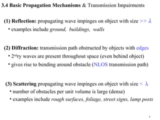
  • 1. 1 3.4 Basic Propagation Mechanisms & Transmission Impairments (1) Reflection: propagating wave impinges on object with size >> λ • examples include ground, buildings, walls (2) Diffraction: transmission path obstructed by objects with edges • 2nd ry waves are present throughout space (even behind object) • gives rise to bending around obstacle (NLOS transmission path) (3) Scattering propagating wave impinges on object with size < λ • number of obstacles per unit volume is large (dense) • examples include rough surfaces, foliage, street signs, lamp posts
  • 2. 2 Models are used to predict received power or path loss (reciprocal) based on refraction, reflection, scattering • Large Scale Models • Fading Models at high frequencies  diffraction & reflections depend on • geometry of objects • EM wave’s, amplitude, phase, & polarization at point of intersection
  • 3. 3 3.5 Reflection: EM wave in 1st medium impinges on 2nd medium • part of the wave is transmitted • part of the wave is reflected (1) plane-wave incident on a perfect dielectric (non-conductor) • part of energy is transmitted (refracted) into 2nd medium • part of energy is transmitted (reflected) back into 1st medium • assumes no loss of energy from absorption (not practically) (2) plane-wave incident on a perfect conductor • all energy is reflected back into the medium • assumes no loss of energy from absorption (not practically)
  • 4. 4 (3) Γ = Fersnel reflection coefficient relates Electric Field intensity of reflected & refracted waves to incident wave as a function of: • material properties, • polarization of wave • angle of incidence • signal frequency boundary between dielectrics (reflecting surface) reflected wave refracted wave incident wave
  • 5. 5 (4) Polarization: EM waves are generally polarized • instantaneous electric field components are in orthogonal directions in space represented as either: (i) sum of 2 spatially orthogonal components (e.g. vertical & horizontal) (ii) left-handed or right handed circularly polarized components • reflected fields from a reflecting surface can be computed using superposition for any arbitrary polarizationE|| E⊥
  • 6. 6 3.5.1 Reflection from Dielectrics • assume no loss of energy from absorption EM wave with E-field incident at ∠θi with boundary between 2 dielectric media • some energy is reflected into 1st media at ∠θr • remaining energy is refracted into 2nd media at ∠θt • reflections vary with the polarization of the E-field plane of incidence reflecting surface= boundary between dielectrics θi θr θt plane of incidence = plane containing incident, reflected, & refracted rays
  • 7. 7 Two distinct cases are used to study arbitrary directions of polarization (1) Vertical Polarization: (Evi) E-field polarization is • parallel to the plane of incidence • normal component to reflecting surface (2) Horizontal Polarization: (Ehi) E-field polarization is • perpendicular to the plane of incidence • parallel component to reflecting surface plane of incidence θi θr θt Evi Ehi boundary between dielectrics (reflecting surface)
  • 8. 8 • Ei & Hi = Incident electric and magnetic fields • Er & Hr = Reflected electric and magnetic fields • Et = Transmitted (penetrating) electric field Hi Hr Ei Er θi θr θt ε1,µ1, σ1 ε2,µ2, σ2 Et Vertical Polarization: E-field in the plane of incidence Hi HrEi Er θi θr θt ε1,µ1, σ1 ε2,µ2, σ2 Et Horizontal Polarization: E-field normal to plane of incidence
  • 9. 9 (1) EM Parameters of Materials ∀ε = permittivity (dielectric constant): measure of a materials ability to resist current flow • µ = permeability: ratio of magnetic induction to magnetic field intensity • σ = conductance: ability of a material to conduct electricity, measured in Ω-1 dielectric constant for perfect dielectric (e.g. perfect reflector of lossless material) given by ε0 = 8.85 ×10⁻¹² F/m
  • 10. 10 often permittivity of a material, ε is related to relative permittivity εr ε = ε0 εr lossy dielectric materials will absorb power  permittivity described with complex dielectric constant (3.18)where ε’ = fπ σ 2 (3.17)ε = ε0 εr -jε’ highly conductive materials  ∀εr & σ are generally insensitive to operating frequency r f εε σ 0 < • ε0 and εr are generally constant • σ may be sensitive to operating frequency
  • 11. 11 Material εr σ σ/εrε0 f (Hz) Poor Ground 4 0.001 2.82 ×10⁷ 108 Typical Ground 15 0.005 3.77 ×10⁷ 108 Good Ground 25 0.02 9.04 ×10⁷ 108 Sea Water 81 5 6.97 ×10⁹ 108 Fresh Water 81 0.001 1.39 ×10⁶ 108 Brick 4.44 0.001 2.54 ×10⁷ 4⋅109 Limestone 7.51 0.028 4.21 ×10⁸ 4⋅109 Glass, Corning 707 4 0.00000018 5.08 ×10³ 106 Glass, Corning 707 4 0.000027 7.62 ×10⁵ 108 Glass, Corning 707 4 0.005 1.41 ×10⁸ 1010
  • 12. 12 • because of superposition – only 2 orthogonal polarizations need be considered to solve general reflection problem Maxwell’s Equation boundary conditions used to derive (3.19-3.23) Fresnel reflection coefficients for E-field polarization at reflecting surface boundary • Γ|| represents coefficient for || E-field polarization • Γ⊥ represents coefficient for ⊥ E-field polarization (2) Reflections, Polarized Components & Fresnel Reflection Coefficients
  • 13. 13 Fersnel reflection coefficients given by (i) E-field in plane of incidence (vertical polarization) Γ|| = it it i r E E θηθη θηθη sinsin sinsin 12 12 + − = (3.19) (ii) E-field not in plane of incidence (horizontal polarization) Γ⊥ = ti ti i r E E θηθη θηθη sinsin sinsin 12 12 + − = (3.20) ηi = intrinsic impedance of the ith medium • ratio of electric field to magnetic field for uniform plane wave in ith medium • given by ηi = ii εµ
  • 14. 14 velocity of an EM wave given by ( ) 1− µε boundary conditions at surface of incidence obey Snell’s Law ( ) ( ) )90sin()90sin( 222111 θεµθεµ −=− (3.21) θi = θr (3.22) Er = Γ Ei (3.23a) Et = (1 + Γ )Ei (3.23b) Γ is either Γ|| or Γ⊥ depending on polarization • | Γ | ≈ 1  for a perfect conductor, wave is fully reflected • | Γ | ≈ 0  for a lossy material, wave is fully refracted         −−= − )90sin(sin90 2 11 it θ η η θ
  • 15. 15 • radio wave propagating in free space (1st medium is free space) • µ1 = µ2 Γ|| = irir irir θεθε θεθε 2 2 cossin cossin −+ −+− (3.24) Γ⊥ = iri iri θεθ θεθ 2 2 cossin cossin −+ −− (3.25) Simplification of reflection coefficients for vertical and horizontal polarization assuming: Elliptically Polarized Waves have both vertical & horizontal components • waves can be depolarized (broken down) into vertical & horizontal E-field components • superposition can be used to determine transmitted & reflected waves
  • 16. 16 (3) General Case of reflection or transmission • horizontal & vertical axes of spatial coordinates may not coincide with || & ⊥ axes of propagating waves • for wave propagating out of the page  define angle ∠θ measured counter clock-wise from horizontal axes spatial horizontal axis spatial vertical axis θ ⊥ || orthogonal components of propagating wave
  • 17. 17 ↔vertical & horizontal polarized components components perpendicular & parallel to plane of incidence Ei H , Ei V Ed H , Ed V • Ed H , Ed V = depolarized field components along the horizontal & vertical axes • Ei H , Ei V = horizontal & vertical polarized components of incident wave relationship of vertical & horizontal field components at the dielectric boundary Ed H, Ed V Ei H , Ei V = Time Varying Components of E-field       =      i v i H C T d v d H E E RDR E E (3.26) - E-field components may be represented by phasors
  • 18. 18 for case of reflection: • D⊥⊥ = Γ⊥ • D|| || = Γ|| for case of refraction (transmission): • D⊥⊥ = 1+ Γ⊥ • D|| || = 1+ Γ|| R =       − θθ θθ cossin sincos , θ = angle between two sets of axes DC =       ⊥⊥ ||||0 0 D D R = transformation matrix that maps E-field components DC = depolarization matrix
  • 19. 19 1.0 0.8 0.6 0.4 0.2 0.0 0 10 20 30 40 50 60 70 80 90 |Γ||| εr=12 εr=4 angle of incidence (θi) Brewster Angle (θB) for εr=12 vertical polarization (E-field in plane of incidence) for θi < θB: a larger dielectric constant  smaller Γ|| & smaller Er for θi > θB: a larger dielectric constant  larger Γ|| & larger Er Plot of Reflection Coefficients for Parallel Polarization for εr= 12, 4
  • 20. 20 εr=12 εr=4 |Γ⊥|1.0 0.9 0.8 0.7 0.6 0.5 0.4 0.3 0 10 20 30 40 50 60 70 80 90 angle of incidence (θi) horizontal polarization (E-field not in plane of incidence) for given θi: larger dielectric constant  larger Γ⊥ and larger Er Plot of Reflection Coefficients for Perpendicular Polarization for εr= 12, 4
  • 21. 21 e.g. let medium 1 = free space & medium 2 = dielectric • if θi  0o (wave is parallel to ground) • then independent of εr, coefficients |Γ⊥|  1 and |Γ|||  1 Γ|| = 1 cos cos cossin cossin 2 2 0 2 2 = − − = −+ −+− = ir ir irir irir i θε θε θεθε θεθε θ Γ⊥ = 1 cos cos cossin cossin 2 2 0 2 2 −= − −− = −+ −− = ir ir iri iri i θε θε θεθ θεθ θ thus, if incident wave grazes the earth • ground may be modeled as a perfect reflector with |Γ| = 1 • regardless of polarization or ground dielectric properties • horizontal polarization results in 180° phase shift
  • 22. 22 3.5.2 Brewster Angle = θB • Brewster angle only occurs for vertical (parallel) polarization • angle at which no reflection occurs in medium of origin • occurs when incident angle θi is such that Γ|| = 0  θi = θB • if 1st medium = free space & 2nd medium has relative permittivity εr then (3.27) can be expressed as 1 1 2 − − r r ε ε sin(θB) = (3.28 ) sin(θB) = 21 1 εε ε + (3.27 ) θB satisfies
  • 23. 23 e.g. 1st medium = free space Let εr = 4  116 14 − − sin(θB) = = 0.44 θB = sin-1 (0.44) = 26.6o Let εr = 15  115 115 2 − − sin(θB) = = 0.25 θB = sin-1 (0.25) = 14.5o
  • 24. 24 3.6 Ground Reflection – 2 Ray Model Free Space Propagation model is inaccurate for most mobile RF channels 2 Ray Ground Reflection model considers both LOS path & ground reflected path • based on geometric optics • reasonably accurate for predicting large scale signal strength for distances of several km • useful for - mobile RF systems which use tall towers (> 50m) - LOS microcell channels in urban environments Assume • maximum LOS distances d ≈ 10km • earth is flat
  • 25. 25 Let E0 = free space E-field (V/m) at distance d0 • Propagating Free Space E-field at distance d > d0 is given by E(d,t) =             − c d tw d dE ccos00 (3.33) • E-field’s envelope at distance d from transmitter given by |E(d,t)| = E0 d0/d (1) Determine Total Received E-field (in V/m) ETOT ELOS Ei Er = Eg θi θ0 d ETOT is combination of ELOS & Eg • ELOS = E-field of LOS component • Eg = E-field of ground reflected component • θi = θr
  • 26. 26 d’ d” ELOS Ei Egθi θ0 d ht hr E-field for LOS and reflected wave relative to E0 given by: and ETOT = ELOS + Eg ELOS(d’,t) =             − c d tw d dE c ' cos ' 00 (3.34) Eg(d”,t) =             − c d tw d dE Γ c " cos " 00 (3.35) assumes LOS & reflected waves arrive at the receiver with - d’ = distance of LOS wave - d” = distance of reflected wave
  • 27. 27 From laws of reflection in dielectrics (section 3.5.1) θi = θ0 (3.36) Eg = Γ Ei (3.37a) Et = (1+Γ) Ei (3.37b) Γ = reflection coefficient for ground Eg d’ d” ELOS Ei θi θ0 Et
  • 28. 28 resultant E-field is vector sum of ELOS and Eg • total E-field Envelope is given by |ETOT| = |ELOS + Eg| (3.38) • total electric field given by +            − c d tw d dE c ' cos ' 00             −− c d tw d dE c " cos " )1( 00 (3.39)ETOT(d,t) = Assume i. perfect horizontal E-field Polarization ii. perfect ground reflection iii. small θi (grazing incidence)  Γ ≈ -1 & Et ≈ 0 • reflected wave & incident wave have equal magnitude • reflected wave is 180o out of phase with incident wave • transmitted wave ≈ 0
  • 29. 29 • path difference ∆ = d” – d’ determined from method of images ( ) ( ) 2222 dhhdhh rtrt +−−++∆ = (3-40) if d >> hr + ht  Taylor series approximations yields (from 3-40) ∆ ≈ d hh rt2 (3-41) (2) Compute Phase Difference & Delay Between Two Components ELOS d d’ d”θi θ0 ht hr ∆h ht+hr Ei Eg
  • 30. 30 once ∆ is known  we can compute • phase difference θ∆ = c wc⋅∆ = ∆ λ π2 (3-42) • time delay τd = cfc π θ 2 ∆ = ∆ (3-43) As d becomes large  ∆ = d”-d’ becomes small • amplitudes of ELOS & Eg are nearly identical & differ only in phase "' 000000 d dE d dE d dE ≈≈ (3.44) if Δ = λ/n  θ∆ = 2π/n0 π 2π λ Δ
  • 31. 31 (3) Evaluate E-field when reflected path arrives at receiver ( )0cos " )1( '" cos ' 0000 d dE c dd w d dE c −+            − (3.45)ETOT(d,t)|t=d”/c = t = d”/creflected path arrives at receiver at       −      ∆ 1cos00 c w d dE c≈ ( )[ ]1cos00 −∆θ d dE = ( )[ ]100 −∠ ∆θ d dE =
  • 32. 32 (3.46) ( )( )∆∆ +−      θθ 22 2 00 sin1cos d dE =( ) ∆∆       +−      θθ 2 2 002 2 00 1 sin d dE cos d dE |ETOT(d)|= = =             ∆ 2 sin2 00 θ d dE ∆−      θcos2200 d dE (3.47) (3.48) ETOT " 00 d dE 'd dE 00 θ∆ Use phasor diagram to find resultant E-field from combined direct & ground reflected rays: (4) Determine exact E-field for 2-ray ground model at distance d
  • 33. 33 As d increases  ETOT(d) decreases in oscillatory manner • local maxima 6dB > free space value • local minima ≈ -∞ dB (cancellation) • once d is large enough  θΔ < π & ETOT(d) falls off asymtotically with increasing d -50 -60 -70 -80 -90 -100 -110 -120 -130 -140 101 102 103 104 m fc = 3GHz fc = 7GHz fc = 11GHz Propagation Loss ht = hr = 1, Gt = Gr = 0dB
  • 34. 34 if d satisfies 3.50  total E-field can be approximated as: k is a constant related to E0 ht,hr, and λ rad d hh rt 3.0 22 2 1 2 <≈ ∆ =∆ λ π λ πθ (3.49) d > (3.50) λλ π rtrt hhhh 20 3 20 ≈this implies For phase difference, θ∆ < 0.6 radians (34o ) sin(0.5θ∆ ) ≈ θ∆             ∆ 2 2 00 θ d dE |ETOT(d)| ≈ e.g. at 900MHz  if ∆ < 0.03m  total E-field decays with d2 2 00 22 d k d hh d dE rt ≈      λ π (3.51)ETOT(d) ≈ V/m
  • 35. 35 Received Power at d is related to square of E-field by 3.2, 3.15, & 3.51 Pr(d) = (3.52b)      = π λ ππ 4120 )( 120 )( 222 0 rR e GdE A dE Pr(d) = 4 22 d hh GGP rt rtt (3.52a) • received power falls off at 40dB/decade • receive power & path loss become independent of frequency rthhif d >>
  • 36. 36 Path Loss for 2-ray model with antenna gains is expressed as: • for short Tx-Rx distances use (3.39) to compute total E field • evaluate (3.42) for θ∆ = π (180o )  d = 4hthr/λ is where the ground appears in 1st Fresnel Zone between Tx & Rx - 1st Fresnel distance zone is useful parameter in microcell path loss models PL(dB) = 40log d - (10logGt + 10logGr + 20log ht + 20 log hr ) (3.53) PL = 1 4 22 −       = d hh GG P P rt rt r t • 3.50 must hold