1. Elec3017:
Electrical Engineering Design
Chapter 8: Electromagnetic
Compatibility
A/Prof D. S. Taubman
August 29, 2006
1 Purpose of this Chapter
Electromagnetic compatibility refers to the ability of an electronic product to
operate correctly within its environment. There are two aspects to this: 1) the
product must be able to operate correctly even in the presence of electromagnetic
interference (EMI) from other electrical appliances; and 2) the product must not
itself generate undue electromagnetic interference.
The first aspect addresses the fact that EMI is unavoidable, so that electronic
products must be designed in such a way that they do not fall victim to its
effects. We take this aspect up first in Section 2. The second aspect addresses
the fact that all electronic products are sources of EMI. Inserting products which
produce undue levels of EMI into the environment may make it impossible for
other products to function. For this reason, acceptable levels of EMI generation
are the subject of regulatory standards, rendering the sale of non-conforming
products illegal. We consider methods to minimize generated EMI in Section
4. As we shall see, many of the methods which reduce susceptibility to EMI
(taking the perspective of a victim) also reduce the amount of generated EMI
(taking the perspective of a source).
Most likely, you will approach this subject with the view that electromag-
netic interference consists of unwanted RF emissions. Certainly this is true,
but EMI occurs also at very low frequencies, right down to DC. At very high
frequencies, EMI may be radiated wirelessly, while at low frequencies we will
be more interested in EMI which is conducted through wires. This includes the
mains wiring which is shared by appliances in your home.
Failure to pay proper attention to electromagnetic compatibility may have
serious adverse consequences. Here are some of the potential consequences, in
order of increasing seriousness:
• Poor or lost reception in wireless applications;
1
2. c
°Taubman, 2006 ELEC3017: Electromagnetic Compatibility Page 2
• Corruption of analog or digital data on transmission lines;
• Malfunction of medical electronic equipment;
• Malfunction of automotive microprocessor control systems; or
• Inadvertent detonation of explosive devices.
Since electromagnetic interference is a complex, multi-faceted topic, with
this brief chapter we cannot hope to make you an expert. Our treatment will
focus mostly upon basic principles of good design. We begin in Section 2 with
a discussion of basic principles to minimize your susceptibility to EMI. This is
followed by Section 3, which is concerned exclusively with the problem of com-
municating information over transmission lines. Transmission lines effectively
extend our electronic circuits over quite some distance, making them particu-
larly vulnerable to EMI. The perspective in both of these sections is that EMI
happens and all we can do is minimize our susceptibility to it. In Section 4, we
look at the techniques to minimize the amount of EMI which you produce.
2 Methods to Avoid Being a Victim of EMI
It is important to realize that EMI occurs not only between electronic prod-
ucts, but also within an electronic product. That is, circuit elements from one
part of the product interfere with other parts of the product. The material
in the present section is concerned with both internal and external EMI. The
material is organized into three sub-sections, which can be classified as primary,
secondary and tertiary levels of control.
2.1 Primary control: components and Layout
There are three types of electromagnetic coupling with which we are principally
concerned at the level of circuit layout. These are covered under the following
headings.
2.1.1 Inductive coupling
We use this term to refer to the susceptibility of conductive loops in your cir-
cuit to alternating magnetic fields. The situation is illustrated in Figure 1.
The alternating magnetic fields in question may be generated by nearby cir-
cuit elements within the same product, or they may be due to propagating RF
electromagnetic waves from more distant sources1 . In either case, an induced
electromotive force (EMF) E = dΦ is generated in the circuit loop, where the
dt
magnetic flux Φ is proportional to the total area contained within the loop. The
primary defense, therefore, against inductive coupling is to keep sensitive signal
conductors as straight as possible. This can be more difficult than you might
1 At a fundamental level, there is no difference between these two sources, since uncontained
alternating magnetic fields always give rise to propagating EM waves.
3. c
°Taubman, 2006 ELEC3017: Electromagnetic Compatibility Page 3
circuit loop
enclosed
flux, Φ
Figure 1: Inductive coupling: alternating magnetic fields create an EMF in
circuit loops. These may be difficult to avoid due to layout constraints. The
figure shows two IC’s with interconnected pins. These might be opamps with an
output from one opamp connected to multiple inputs on other opamps.
X
Separation, d
Y
Overlapping area, A
Figure 2: Capacitive coupling between conductors X and Y.
think, particularly when signal lines are used to connect multiple components,
as suggested by Figure 1. It is also worth noting that electronic components
themselves are part of the circuit. Their packages and leads may well form
or contribute to circuit loops, which are susceptible to inductive coupling. Of
course, the worst offenders are likely to be inductors and transformers.
2.1.2 Capacitive coupling
Capacitive coupling can occur between any two closely spaced conductors, X
and Y , as shown in Figure 2. The capacitance formed between such conductors is
roughly proportional to A , where A is the shared surface area of the conductors
d
and d is their separation. In practice, of course, both the area and separation
may vary from point to point, so this formula serves only as a guide to help you
minimize capacitive coupling. Evidently, the two most obvious actions you can
take are: 1) minimize the surface area of either or both conductors (i.e., use thin,
short wires); and 2) keep sensitive circuit traces as far away from interference
sources as possible.
An important additional mitigation strategy is to insert a grounded conduc-
tor G, between X and Y . As shown in Figure 3, this replaces the capacitance
between X and Y with two capacitances, one between X and G and another
between Y and G. So long as G has low impedance and is tied to a stable fixed
reference voltage, capacitive currents flowing between Y and G will have very
4. c
°Taubman, 2006 ELEC3017: Electromagnetic Compatibility Page 4
X
G
Y
Figure 3: Decoupling conductors X and Y by inserting an intermediate ground
conductor G. Note the effective capacitances formed between X and G and Y
and G.
little impact on the potential of the ground conductor and hence the capaci-
tive currents flowing between X and G. Similarly, capacitive currents flowing
between X and G will have negligible impact on Y .
There are various ways to implement this strategy in practice. If conductors
X and Y are running parallel to each other on a single side of a printed circuit
board (PCB), you may insert an extra ground trace between them. If conductors
X and Y are on opposite sides of a PCB, the ground conductor G might run
in an internal PCB layer, of a multi-layered PCB — in the extreme case, this
might be an expansive sheet of copper, known as a ground plane. If one or both
of X and Y is a flexible conductor whose position is hard to fix, the ground
conductor G might be a copper mesh which completely encloses one of X or Y
— this is known as a shield.
2.1.3 Conductive coupling and ground planes
One particularly insidious form of electromagnetic coupling occurs when differ-
ent parts of the circuit share conductive paths. We restrict our attention here
to the case where the shared paths correspond to ground or power lines, since
these are the places where problems are most likely to occur.
Figure 4 illustrates the problem of shared power lines. Since the power con-
ductors have non-negligible impedance, the current consumption behaviour of
downstream components introduces voltage drops along both power and ground
lines, which are experienced by upstream components. One way to mitigate this
effect is to use conductors of large cross-sectional area, and hence very low resis-
tance, for power lines. Unfortunately, this is of limited effectiveness in suppress-
ing very high frequency power line transients. The problem is that the power
lines also have appreciable self-inductance which converts current transients into
voltage drops, according to
dI
V =L .
dt
The self inductance of a conductor does not reduce substantially as cross-
sectional area is increased.
For this reason, it is important that you include local capacitors across the
supply rails of components which may consume large or rapidly changing cur-
5. c
°Taubman, 2006 ELEC3017: Electromagnetic Compatibility Page 5
Vcc (+5V)
TTL Buffer opamp TTL Logic
Gnd (0V)
Vee (-5V)
Figure 4: Power and ground lines shared by multiple circuit components, showing
supply currents. Of course, there will be additional currents flowing through
signal lines, not shown here.
Vcc (+5V)
TTL Buffer opamp TTL Logic
Gnd (0V)
Vee (-5V)
Figure 5: Power supply decoupling capacitors.
rents. This is illustrated in Figure 5. These capacitors are commonly known as
decoupling capacitors, or bypass capacitors. Typical values range from 1 nF to
100 nF, depending on the application. For good decoupling of high frequency
power supply transients, ceramic capacitors are generally recommended. Spe-
cial ceramic decoupling capacitors known as monolithic capacitors are commonly
available, with typical values of 22 nF and 100 nF.
Even with decoupling capacitors and low resistance power and ground lines,
appreciable levels of coupling can still occur. Further decoupling can be achieved
by distributing power to your components via a star network, as shown in Fig-
ure 6. In this case, separate circuit components do not share the same power
conductors. In practice, this can be quite difficult to arrange for each individual
circuit component. Moreover, capacitive coupling of different branches in the
star becomes increasingly likely as the complexity of the power distribution net-
work grows. For these reasons, an intermediate solution is normally adopted, in
which sensitive analog components in the circuit sit on one branch in the power
distribution network, with noisy digital components powered from a separate
branch. Such a partitioned system is shown in Figure 7.
6. c
°Taubman, 2006 ELEC3017: Electromagnetic Compatibility Page 6
TTL Buffer
Vcc (+5V) TTL Logic
Gnd (0V)
Vee (-5V)
opamp
Figure 6: Star configuration for distributing power without shared conductors.
TTL Buffer digital TTL Logic
partition
Vcc (+5V) Gnd (0V)
analog
opamp partition opamp
Vee (-5V)
Figure 7: Partitioned power and ground system.
7. c
°Taubman, 2006 ELEC3017: Electromagnetic Compatibility Page 7
The ground reference conductor plays a special role in most circuits, as a
common reference potential shared by many signals. Voltage drops along the
ground conductor may appear to the extent that it is used to carry transient
power supply currents, as discussed above. Voltage drops may also be caused
by larger signal currents. These cannot be mitigated by decoupling capacitors,
since signal line voltages are not generally supposed to be constant. Star and
partitioned ground networks are widely used to combat conducted coupling via
ground lines.
Another commonly employed technique is the use of ground planes. A ground
plane is an expansive sheet of copper, which serves to establish a solid ground
reference potential. The use of ground planes can add to the cost of a printed
circuit board, since they typically consume an entire layer of the board. On
the other hand, ground planes can provide very low resistance. Interestingly,
ground planes can also lower the inductance experienced by ground currents.
One reason for this is that high frequency ground currents will tend to find the
path through the plane which encloses the smallest possible loop area, leading
to lower inductance than is usually achieved by running separate ground tracks
across a PCB.
It is tempting to think that a ground plane will cure all your ground-based
signal coupling problems; this kind of thinking, however, can get you into trou-
ble. The main problem is that ground planes deprive you of control over the
paths which are actually taken by ground currents. This means that high tran-
sient currents produced by line drivers or high speed digital IC’s may intersect
with the ground return paths taken by sensitive analog signals. Since currents
fan out within the ground plane in a complicated fashion, interference is difficult
to avoid and may lead to quite unexpected coupling in high gain analog circuits.
With this in mind, it is best to partition your ground plane into physically sep-
arated regions: one for sensitive analog components; one for less sensitive line
driving components2 ; and one for switching components such as digital IC’s.
These partitioned ground regions can then be connected via a star configura-
tion, as suggested in Figure 7.
2.2 Secondary control: interface filtering
In Section 3, we take up the problem of reliable communication over transmission
lines. At this point, however, we note that the signals arriving at input interfaces
to (or within) your product will generally be corrupted by noise and interference.
These can be substantially suppressed through the use of input filters, whose
purpose is to remove frequency content which lies outside the range of the
signals you are actually expecting to receive. Without input filtering, noise and
interference power may substantially exceed the power of the intended signal
that you are trying to recover. Simple R-C filters are commonly employed,
but more complex multi-pole filters might also be required. If the frequencies
2 This one is optional. Many designs involve only two ground regimes: one for sensitive
signals and one for less sensitive signals with higher slew rates.
8. c
°Taubman, 2006 ELEC3017: Electromagnetic Compatibility Page 8
LM7805 Π filter
SUPPLY + VCC
in out
unregulated ref
regulated
output
input
SUPPLY - GND
Figure 8: Filtering at the output of a regulated power supply to suppress EMI.
involved are not too high (e.g., less than 1 MHz), good input filters can be
constructed with the aid of opamps, so that the only passive elements required
are resistors and capacitors. At very high frequencies, tuned circuits containing
both capacitors and inductors are generally required.
An important source of electromagnetic interference is through mains power
lines. Common sources of EMI on mains power lines include:
• switches;
• appliances with commutated motors (e.g., electric drills, kitchen tools,
vacuum cleaners, etc.);
• electric light dimmers (these introduce strong switching transients part
way through the 50 Hz mains cycle); and
• communication devices which use the mains wiring as a communications
medium.
Interference from such sources can be coupled into your product via its power
supply system. In fact, this can be a significant problem for audio amplification
and mixing equipment. Again, the solution is to filter out unwanted frequency
components, either before or within the regulated power supply system. The use
of resistors and/or active amplifiers (e.g., opamps) in such filters is not generally
appropriate, since these would waste significant amounts of power. For this
reason, high quality power supply filtering generally involves both capacitors
and inductors. A common configuration is the Π filter shown in Figure 8.
2.3 Tertiary control: shielding as a last resort
High frequency radiated EMI can be strongly attenuated by enclosing your
electronic product (or sensitive sub-systems) in metal shielding. To appreciate
the effectiveness of this as a solution, it is important to understand the concept
of skin depth. EM waves with frequency f , propagating through a metal with
conductivity σ, have their amplitude attenuated according to
z
A (z) = A0 e− δ(f,σ) (1)
9. c
°Taubman, 2006 ELEC3017: Electromagnetic Compatibility Page 9
num ber of available
defense deasures
cost of defense
deasures
tim e
Figure 9: Availability and cost of EMI defense measures as the product design
process evolves.
Here, z denotes the propagation distance and
s
ε0 · c2
δ(f, σ) = (2)
σ·π·f
is the skin depth of the metal. At a distance δ (f, σ) into the surface of the
metal, the amplitude is already reduced by 1 , meaning that the RF power is
e
reduced by e−2 ; at two skin depths, the amplitude and power are reduced by
e−2 and e−4 , respectively; and so forth. For effective shielding, two or three
skin depths may be sufficient.
For copper, the ratio σ/ε0 (conductivity divided by the permittivity of free
space) is 6.5 × 10¹⁸ s−1 . Noting that the speed of light is c = 2.998 × 10⁸ m/s,
we find that the skin-depth is given by
√
copp er 6.634 4 × 10⁻² m · Hz
δ (f ) = √
f
At 1 MHz, for example, the skin depth is a mere 66 μm. On the other hand, at
100 Hz, the skin depth is 6.6 mm, which is a very thick sheet of copper indeed.
Evidently, shielding cannot generally protect you from low frequency EMI.
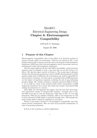
Shielding also adds substantial cost and weight to your product, so it should
be seen as a course of last resort. Shielding is relatively easy to add as an
after-thought, if your design proves overly susceptible to EMI. Other, less costly
measures, however, must be incorporated in earlier stages of the design process.
This relationship between time, cost and available EMI defense mechanisms is
depicted in Figure 9.
3 Transmission Lines and Differential Signalling
In this section we devote special attention to the case of transmission lines.
We use the term transmission line to refer to any wired signalling system for
10. c
°Taubman, 2006 ELEC3017: Electromagnetic Compatibility Page 10
communicating information over distance. This includes wires which link sep-
arate electronic products (e.g., the cabling from a guitar pre-amp to a high
power audio amplifier), as well as signal lines which are used to connect distinct
sub-systems within a single electronic product. What makes transmission lines
particularly important is that they extend over a significant distance, so they
are likely to be exposed to substantial levels of EMI. For this reason, we will
need to develop circuit solutions to minimize the impact of this EMI. Just what
constitutes a significant distance depends upon the application at hand: the
frequencies involved; the sensitivity of the signals; and the expected levels of
electromagnetic interference.
We begin our discussion of transmission lines by considering the various
modes by which EMI may be coupled into a transmission line consisting of two
conductors: an active signal conductor; and a ground conductor. In this con-
text, we show how ground shields can be beneficial when used with appropriate
receiving circuitry. We then turn our attention to differential signalling schemes,
involving two active signal lines.
3.1 Single-ended signalling
Figure 10 illustrates an overly simplistic signalling environment, in which the
transmission line consists of a ground conductor and a single active signal line.
The information (analog or digital) is communicated via the voltage difference
between the active signal line (shown on top) and the ground potential (shown
on the bottom). For simplicity, we think of the transmitter and receiver as
physically distinct electronic products and consider the various ways in which
EMI may find its way into the received signal. The most important of these are
as follows:
Direct inductive coupling: This occurs in the presence of alternating mag-
netic fields, such as those produced by propagating EM waves. The al-
ternating flux Φ1 enclosed by the signal and ground conductors in the
transmission line (see Figure 10) produces an induced EMF, which is su-
perimposed on the desired signal at the receiver.
Capacitive coupling to earth: This occurs when either of the conductors in
the transmission line are sufficiently close to another conducting surface
whose voltage potential is a source of interference. We use the generic
term earth here to refer to this conducting surface. In practice, the close
interfering surface might be the metal case of another electronic product.
Alternatively, it might be a human being, whose body potential is oscil-
lating in response to EM waves (as an antenna) or in response to another
interference source, to which it is capacitively or directly coupled. Ca-
pacitive coupling can occur only if the potential of the nearby interfering
surface oscillates rapidly, or when the separation between the transmission
line and the interfering surface itself oscillates rapidly3 .
3A time varying displacement between conductors produce a time varying capacitance,
11. c
°Taubman, 2006 ELEC3017: Electromagnetic Compatibility Page 11
Conductive coupling via earth: A potentially very serious EMI coupling
modality occurs if transmitter and receiver are both connected to the
mains earth wiring. Many electrical appliances have a metal case which is
directly connected to the mains earth as a safety precaution. In the event
of an electrical fault in the appliance, a large current will flow to earth,
causing a fuse or circuit breaker to open in the local mains breaker box.
This topic is covered more extensively in Chapter 9. All that need be ap-
preciated here is that electronic products which consume significant power
are usually earthed. Internal to the transmitter and receiver, the ground
reference potential is also either directly connected to the earthed case
(and hence to the external mains earth) or else there is strong capacitive
coupling to the case and earth (e.g., through the windings of a transformer
used for power supply isolation). These connections are shown as dashed
lines in Figure 10. They provide a mechanism for the coupling of earth
currents into the signal recovered by the receiver. To see this, note that
earth currents produce potential differences between different points in
the mains earth wiring. These potential differences produce currents in
the transmission line’s ground conductor, which has non-zero resistance
and self inductance. In this way, earth currents produce end-to-end po-
tential differences in the transmission line’s ground conductor, which are
superimposed on the signal recovered by the receiver.
Inductive coupling via earth: Even if no other appliances share the mains
earth wiring path between the transmitter and the receiver, it is still pos-
sible that earth currents appear, producing superimposed waveforms on
the received signal. A major cause of this is the coupling of alternating
magnetic fields into the circuit formed by the transmission line’s ground
conductor and the earth. This is identified in Figure 10 by the magnetic
flux term Φ2 . Even though this is a less direct path for EMI coupling than
that discussed above due to flux term Φ1 , the area enclosed between the
transmission line and the mains earth wiring is usually much greater than
that enclosed between the two conductors in the transmission line itself.
Having examined some of the more significant modes by which EMI may
be coupled into a single-ended transmission line, we now consider methods for
minimizing its impact. The first measure we will consider is the use of shielded
cabling. There are still only two conductors in the transmission line, but one of
these (the ground conductor) consists of a flexible wire mesh which completely
surrounds the inner conductor (the active signal line). This is illustrated in
Figure 11.
Shielding can substantially eliminate direct inductive coupling. To see this,
observe that EMF contributions E1 and E2 depicted in Figure 11 should be
almost identical, assuming that the magnetic field strength varies little between
the top and bottom edges of the cable. These EMF contributions produce
whose stored charge induces a time varying voltage. This mode of coupling, however, is rarely
significant.
12. c
°Taubman, 2006 ELEC3017: Electromagnetic Compatibility Page 12
transmitter receiver
transmission line
dΦ1 / dt
dΦ 2 / dt
earth currents earth
Figure 10: Coupling of electromagnetic interference to a transmission line in-
volving single-ended signalling.
dΦ / dt ε1
dΦ / dt ε2
Figure 11: Shielded cable with one active signal line.
opposite superimposed waveforms on the received signal, so that the inductive
coupling contributions largely cancel.
Shielded cables also largely eliminate capacitive coupling between external
interference potentials (or earth) and the inner conductor. Virtually all ca-
pacitively coupled interference currents flow in the grounded shield, whose im-
pedance is much lower than that of the inner active signal line. Such capacitive
currents can still produce potential differences along the shield conductor, but
their impact is generally much smaller than that of capacitive coupling to the
active signal line, especially considering the non-zero output impedance of the
transmitter’s line driving circuitry.
Apart from providing a low impedance ground conductor, shielded cables do
not inherently provide a solution to the third and fourth EMI coupling modes
described above. To address these, it is necessary to break the ground-earth
circuit. This means that you should not tie the shield to both the transmit-
ter’s ground reference point and the receiver’s ground reference point. To avoid
ambiguity, the convention is to tie only the shield to ground only at the trans-
mitting end, allowing the receiver’s shield potential to float relative to its ground
reference. The receiver then implements a differential amplifier which is sensi-
tive only to the difference between the shield and the active signal line. This
situation is depicted in Figure 12.
As shown in the figure, the shield may still be tied loosely to the receiver’s
ground via a resistor, whose impedance is large compared to that of the shield
conductor. This is important if no other DC path exists between the transmit-
13. c
°Taubman, 2006 ELEC3017: Electromagnetic Compatibility Page 13
receiver
transmitter R2
R1
opamp
VO
R1 R2
Vmax
RG
Vmin
Figure 12: Single-ended transmission line with differential receiver.
ter and receiver’s ground reference point, since the receiver’s differential input
amplifier can only operate over a limited range of input voltages. Interference
waveforms produced by earth currents, and inductive coupling via earth, appear
across this resistor instead of the transmission line’s shield conductor. So long
as the voltages appearing across the resistor do not exceed the common mode
operating range of the receiver’s differential input amplifier, all will be well. The
figure also shows how diode protection may be included to prevent the shield
voltage from exceeding the safe operating range of the receiver’s differential
input amplifier.
Before concluding this sub-section, it is worth noting that a twisted pair can
serve as an inexpensive alternative to shielded cables. As the name suggests, a
twisted pair is just a pair of separately insulated wires which have been twisted
together. Twisting the wires together minimizes inductive coupling effects, since
the magnetic flux enclosed by one twist is roughly cancelled by one twist is
roughly cancelled by that enclosed by the next twist, as we move along the
length of the cable. Again, loose coupling of the ground wire at the receiver,
together with differential amplification, minimize the impact of earth currents
and inductive coupling via earth. Twisted pairs, however, remain much more
susceptible than shielded cables to capacitive coupling of interfering surface
potentials.
3.2 Differential signalling
While the EMI mitigation methods discussed in the previous sub-section can be
quite successful, single-ended signalling strategies still suffer from the drawback
that shield currents flow through one of the two signal conductors (the grounded
shield). These shield currents include the currents produced by capacitively
coupled interfering surface potentials. They also include the residual currents
produced by mains earth noise, which cannot be completely eliminated since
the shield must be tied at least loosely to ground at the receiver — in Figure 12,
this is done by resistor RG and the two common mode voltage limiting diodes.
Since the shield is one of the two information bearing conductors, the voltage
drop produced by shield currents will be superimposed on the received signal.
The solution to this problem is to use two active signal lines, enclosed by a
14. c
°Taubman, 2006 ELEC3017: Electromagnetic Compatibility Page 14
receiver
transmitter R2
R1
opamp
VO
R1 R2
Vmax
RG
Vmin
Figure 13: Transmission line with two active signal lines, enclosed by a separate
grounded shield.
receiver
transmitter R2
R1
opamp
VO
R1 R2
Vmax
RG
Vmin
Figure 14: Similar to Figure 13, except that the two active signal lines are
driven with voltage waveforms v (t) and −v (t), respectively. The transmitter
essentially has two output drivers, one for each signal line, each with the same
output impedance. The sum of the two signal line potentials is equal to the
transmitter’s ground potential.
separate shield. One such configuration is illustrated in Figure 13. Another is
depicted in Figure 14. Both configurations offer excellent immunity to EMI. The
second involves a more complex transmitter which drives one signal line with
the opposite polarity to the other. One advantage of this is that the driving
impedances of both signal lines should be identical, so that they are affected
roughly equally by residual EMI coupling. A second advantage of the differential
signalling strategy in Figure 14 is that any EMI radiated by one active signal
line is roughly cancelled by the EMI radiated by the other active signal line —
see Section 4.
With either of the configurations shown in Figures 13 and 14, the main
modes of potential EMI coupling are as follows:
Differential inductive coupling: This occurs in the presence of alternating
magnetic fields, when the alternating magnetic flux enclosed between the
two active signal lines generates an EMF which is superimposed on the
received signal. Fortunately, the presence of a separate shield significantly
reduces the levels of high frequency EM radiation to which the active
signal lines are subjected, in accordance with equations (1) and (2). To
further mitigate against differential inductive coupling, the active signal
15. c
°Taubman, 2006 ELEC3017: Electromagnetic Compatibility Page 15
lines can be twisted together so that the EMF’s induced in alternate twists
have opposing amplitudes.
Impedance and length mismatches: In principle, EMI should affect both
of the active signal lines identically, so that the difference between their
signal voltages remains unaffected. This is the reason for including a differ-
ential amplifier at the receiver. One example which we have not yet men-
tioned is antenna mode coupling. When suitably aligned, the alternating
electric fields associated with propagating EM waves induce longitudinal
currents in both of the active signal lines, acting as antennae. If the two
active signal lines have different impedances (different transmitter driving
impedances or different receiver input impedances), a differential voltage
will be superimposed on the received signal. A similar effect occurs if the
active signal lines have different lengths.
Capacitive coupling from the shield: Although the grounded shield pro-
tects the active signal lines from external capacitive coupling, it cannot
protect them from itself. If significant shield currents flow in response
to external sources of interference, these will produce voltage drops along
the shield which can be capacitively coupled into the internal signal lines.
Any differences in the levels of capacitive coupling, or mismatches in the
impedance associated with the two signal lines, can produce interference
components in the differential waveform presented to the receiver. In
view of this, you are still strongly discouraged from connecting the shield
to both the transmitter’s and the receiver’s ground reference point. As
in the single-ended case, it is always best to tie the shield only loosely
to ground at the receiving end. At the transmitting end, the shield is
connected directly to ground.
3.3 EMI Suppression Baluns
A useful course of last resort in suppressing EMI on transmission lines is the
ferrite balun. Baluns are just small inductor/transformer cores, whose original
main purpose was the construction of impedance matching transforms for analog
video applications. With the advance of high frequency electronics, however,
baluns are seeing greater use in EMI suppression. The idea is to wind some
number of turns (typically only one) of the transmission cable around the ferrite
core. Split balun cores make it possible to do this without actually disconnecting
any of the leads.
It is important to make sure that all conductors involved in the transmission
line are wound around the balun former together. This means that the EMF’s
induced by magnetic flux in the core should be identical in all signal lines,
so that they do not appear as superimposed signal content. These induced
EMF’s appear only when a net current flows in the cable, which is exactly what
happens when currents circulate in the path formed by the ground conductor
(or shield) and earth — see Figure 10. As mentioned, the generated EMF does
not superimpose any net differential signal at the receiver, but the resulting
16. c
°Taubman, 2006 ELEC3017: Electromagnetic Compatibility Page 16
inductance does serve to raise the impedance of the ground/shield conductor,
allowing potential differences between the receiver and the transmitter to be
bridged without excessive currents.
At very high frequencies, eddy currents in the ferrite core become large,
producing significant power losses. Components which lose power are equivalent
to resistors from a circuit model perspective. Resistive losses in an inductor
are not normally desirable. For EMI suppression, however, this is actually a
desirable phenomenon. Very high frequency components are absorbed in the
ferrite core, which reduces the amount of EM radiation which can be emitted
by the transmission line.
4 Methods to Avoid Being a Source of EMI
In this section, we are concerned with methods for minimizing the amount of
EMI that an electronic product produces. As in Section 2, we can divide the
various mitigation strategies into primary, secondary and tertiary methods. Pri-
mary methods relate to the choice of circuit components and layout; this is the
topic of Section 4.1 below. Secondary methods control the EMI emitted at the
interfaces between sub-systems or products; this is the topic of Section 4.2. As
before, tertiary methods involve shielding. Taking the perspective of a victim,
Section 2.3 discussed shielding for sensitive sub-systems and products. Taking
the perspective of an EMI source, the same arguments show that shielding can
be used to contain or absorb sources of electromagnetic interference. Due to
the symmetry of the source and victim problems, there is no need to consider
tertiary mitigation methods again in this section.
4.1 Primary control: components and layout
Many of the methods described in Section 2.1, for mitigating EMI as a victim,
also reduce the amount of EMI which a circuit produces. In particular, the
following principles should be applied:
Avoid circuit loops with high dI/dt: Current flowing in loops generates a
magnetic field. When the current alternates, an alternating magnetic flux
is produced in other parts of the circuit and external electronic products
leading to inductive coupling of EMI. In fact, the alternating magnetic field
is an origin of propagating EM waves. Therefore, you should endeavour
to avoid loops when laying out conductors for signals with strong high
frequency components.
Avoid large conductor surfaces with high dV /dt: Conductors with large
surface areas can be the source of capacitively coupled EMI. Of course,
this is relevant only to the extent that the conductor’s electric potential
contains strong high frequency components. Large surface areas arise in
the context of long conductors, as well as wide conductors.
17. c
°Taubman, 2006 ELEC3017: Electromagnetic Compatibility Page 17
Avoid sharing conductive paths with sensitive signals: Conductive
coupling through shared power or ground paths has been adequately
discussed already in Section 2.1.
In addition to the above-mentioned points, it is worth noting that non-
linearities in electronic components present a source of unintended high (or
low) frequency components. As a simple example, consider a sinusoidal volt-
age waveform applied to a component (e.g., a resistor) with a square-law non-
linearity; this non-linearity produces currents with frequency components at
twice the source frequency and at DC. In general, non-linearities allow for inter-
modulation of the various frequency components present in your designed prod-
uct. These modulation terms may escape the EMI mitigation measures you
design for the principle frequency components in your circuit.
4.2 Secondary control: interface filtering
In Section 2.2, we noted the importance of filtering signal and power supply
inputs to your product, so as to remove unwanted noise and interference com-
ponents which lie outside the frequency range of interest. In some cases, a
simple R-C circuit is sufficient, in others power efficient inductor-capacitor filter
networks might be required. From the perspective of an EMI source, filtering
is also important.
For generated signals, such as those sent over transmission lines, the purpose
of filtering is to minimize unwanted frequency content produced by the output
driver. When the signals are digital, the chief cause of unwanted high frequency
content is unnecessarily high slew rates between the low and high logic voltage
levels. Slew rates in digital transmission lines should therefore be carefully
controlled. A simple R-C filter may suffice. Alternatively, the line driver’s
current driving (pulling and pushing) capabilities should be matched to the
capacitive load imposed by the transmission line or an explicit load capacitor.
If high slew rates are unavoidable over long transmission lines, a differential
line driving strategy can be employed, as shown in Figure 14. In this case, the
EMI generated by each of the two signal lines should roughly cancel. Techniques
such as these are already starting to enter into the design of high speed memory
buses for digital applications.
Power supplies in electronic products are also a source of considerable EMI
on the mains power lines. Π filters, such as that shown in Figure 8, serve both to
minimize susceptibility to external EMI sources and also to minimize the amount
of EMI which escapes from your circuit into the mains. The rectification process
itself, however, produces strong current switching transients at 100 Hz (for a
50 Hz mains power system). For high power rectifiers, input filtering may be
required to smooth out these switching transients. This generally requires the
use of inductors, as well as capacitors. Figure 15 illustrates one simple power
conditioning filter.
18. c
°Taubman, 2006 ELEC3017: Electromagnetic Compatibility Page 18
Power LM7805
Conditioning Filter VCC
in out
regulated output
mains power input ref
GND
Figure 15: Mains filtered power regulator to reduce EMI emissions to the mains.
5 Regulatory Issues
Acknowledgement: This final section is taken in large part from:
“Design for Electromagnetic Compatibility,” lecture notes prepared by R.
H. Mondel, W. H. Holmes and A. P. Bradley.
A strong regulatory framework exists in all western countries, to control levels
of EMI produced by saleable products (source perspective), as well as the abil-
ity of certain types of products to operate within an environment containing
prescribed levels of EMI (victim perspective).
In Australia, this is administered by the Australian Communications Au-
thority (ACA), which was formed on 1 July 1997 as a merger between AUSTEL
(Australian Telecommunications Authority), which was the telecommunications
industry regulator, and SMA (Spectrum Management Agency), which was re-
sponsible for radio frequency spectrum management and radio communications
licensing.
In the USA, the relevant standards are administered by the FCC (Federal
Communications Commission), while in Europe they are administered mainly
by the IEC (International Electrotechnical Commission).
In Australia, complying equipment receives a C-tick. The equivalent in Eu-
rope is the CE mark. There are severe penalties for placing non-complying
equipment on the market in all countries.
Most of the standards attempt to control electromagnetic emissions. There
are also some standards (especially in Europe) which specify levels of immunity
of equipment to incidental EMI from other sources. These are especially rel-
evant if the equipment is safety critical (e.g., medical electronics and aviation
electronics). There are specialized firms which can carry out tests of compliance.
The main Australian standards are summarized in Table 1.
19. c
°Taubman, 2006 ELEC3017: Electromagnetic Compatibility Page 19
Table 1: Regulatory standards governing electromagnetic compatibility in Aus-
tralia.
Standard EMC/EMI Products Covered
AS1044:1992 Emission Household electrical appliances, portable
power tools and similar
AS2064,1&2:1992 Emission Industrial, scientific and medical radio
frequency equipment
AS3548:1992 Emission Information technology equipment
AS4052:1992 Emission Microwave ovens for frequencies above 1
GHz
AS1053:1992 Emission Sound and television broadcast receivers
and associated equipment
AS2557:1992 Emission Vehicles, motor boats and spark ignited
engine driven motors
AS4051:1994 Emission Electrical lighting and similar products
AS4251:1994 Emission Generic emission standards
AS4053:1992 Immunity Sound and television broadcast receivers
and associated equipment
AS4252:1992 Immunity Generic immunity standard