2006 Pisarski Report on Commuting in America

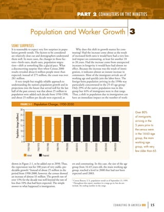
1. PART 2 COMMUTERS IN THE NINETIES
Population and Worker Growth 3
SOME SURPRISES
It is reasonable to expect very few surprises in popu- Why does this shift in growth matter for com-
lation growth trends. The factors to be considered muting? Had the increase come about as the result
are relatively clear cut and demographers understand of increased birth rates it would have had a very lim-
them well. In most cases, the changes in those fac- ited impact on commuting, at least for another 18
tors—birth rates, death rates, population migra- to 20 years. Had the increase come from unexpected
tion—shift at something like a glacial pace. What increases in longevity it would have had almost no
a disconcerting surprise then when Census 2000 effect. Because the increase was the result of immi-
results revealed about 6 million people more than gration, it indicates almost an instant increase in
expected; instead of 275 million, the count was over commuters. Most of the immigrant arrivals are of
281 million. working age and quickly join the labor force. The
A very simple but roughly reliable approach to foreign-born population arriving in the 1990s was
understanding the nation’s population growth and its particularly concentrated in the 25-45 age group.7
projections into the future that served well for the last Only 29% of the native population was in this
half of the past century was that about 25 million in group but 44% of immigrants were in that range.
population were added each decade from 1950-1990, Thus, a shift in population due to immigration can
and about 25 million per decade were expected, as have an immediate impact on the number of work-
FIGURE 2-1 Population Change, 1950-2050
30
Over 80%
Population change (millions)
25
of immigrants
20 arriving in the
15 5 years prior to
the census were
10
in the 16-65 age
5
group, the main
0 working age
2040-2050
2030-2040
1970-1980
1990-2000
2010-2020
1950-1960
1980-1990
1960-1970
2020-2030
2000-2010
group, with very
few older than 65.
Actual Projected
shown in Figure 2-1, to be added out to 2050. Thus, ers and commuting. In this case, the size of the age
the expectation was for 100 years of very stable, pre- group from 16-65 years old, the main working age
dictable growth.6 Instead of about 25 million in the group, reached a level in 2000 that had not been
period from 1990-2000, however, the census showed expected until 2003.
an increase of almost 33 million. The growth rate of
over 13% for the decade was well beyond the rate of 6
Census Bureau, U.S. population trends as of September 13, 1999.
less than 10% that had been expected. The simple 7
Throughout this report, numbers in a range go to, but do not
answer to what happened is immigration. include, the ending number in the range.
C O M M U T I N G I N A M E RI C A III | 15

2. centage terms, was expected (Commuting in America
TABLE 2-1 Worker and Population Increase, 1950-2000
II earmarked 1990 as the turning point that signaled
Total Workers Worker Increase Worker Increase Population the end of the worker boom). However, many are
Year
(Millions) (Millions) (%) Increase (%) hard-pressed to understand the sharper-than-expected
1950 58.9 N/A N/A N/A declines, particularly given the larger-than-expected
increases in immigrants who largely were of working
1960 65.8 6.9 11.7 18.5
age. This situation, critical to commuting, will be
1970 78.6 12.8 19.5 13.3 discussed later in this chapter.
1980 96.7 18.1 23.0 11.4 Another point of note in the table is that the
1990 115.1 18.4 19.2 9.7 30-year decline in the rate of population growth as
the baby boom waned took a sharp reversal in 2000
2000 128.3 13.2 11.5 13.2
and returned to the growth rates of the 1970s. Since
Overall Change 69.4 117.8 86.0 2000, worker growth has been quite limited given
the events of 9/11 and the recession that followed.
Between 2000 and 2003, only 1.4 million work-
TABLE 2-2 Workers Age 65 and Older ers were added, about a 1.1% increase, according
to the American Community Survey (ACS). In
Age Group 1990 2000 Change 2004, Bureau of Labor Statistics (BLS) employment
65- 75 2,947,744 3,305,563 357,819 statistics showed worker growth surged, adding 1.7
75+ 549,718 942,575 392,857 million from December 2003 to December 2004,
but were still an anemic 2.4% growth since 2000.
65+ 3,497,462 4,248,138 750,676
The worker/population ratio of 62.4 was the same at
the end of 2004 as at the start of the year.
A key concern for commuting is the rate of
Perhaps the best example of the effects of immi- growth within the work-age segment of the popula-
gration is the pre–Census 2000 projections for the tion (ages 16-65). BLS has traditionally used 16
number of 18-year-olds, a useful indicator of new or over as their base measure of the labor force age
labor force arrivals. According to projections, this group, but in the coming years that approach may
age group, which had dropped below 4 million after prove misleading, as the baby boom ages and the
1990, would not reach 4 million again until 2008; share of population over 65 surges. The key point,
in fact, 4 million was reached in 2000. and one to monitor carefully in the future, is that in
2000 only 3.3% of workers were age 65 and older,
not much greater than the 3% registered for 1990.
PARALLEL LABOR FORCE TRENDS The population at work among those 65 and older
The boom in workers can be measured by the period rose by roughly 750,000 from 3.5 million in 1990 to
from 1970-1990 when the rates of increase in workers 4.25 million in 2000, about half of the growth com-
exceeded population increase, as seen in Table 2-1. ing from those age 75 and older as shown in Table
Note also that in the overall period from 1950-2000, 2-2. The number of workers age 65 and older rose by
workers in the population more than doubled. All of over 21% in the period while the population in that
this said, the sharp decline in the number and the rate group only rose about 12%. As that group’s share of
of growth in workers in the 1990s comes as another the population increases sharply after 2010, a key
demographic surprise. Some decline, certainly in per- question for commuting will be the extent to which
FIGURE 2-2 Workers by Age Group
50
Worker Nonworker
40
Workers (millions)
30
20
10
0
16-25 25-35 35-45 45-55 55-65 65-75 75+
Age group
16 | COMMUTING IN AMERICA III

3. TABLE 2-3 Population Growth Rates by Age Group, 1990-2000
Age Group 1990 (Millions) 2000 (Millions) Change (%) 1990 Distribution (%) 2000 Distribution (%)
< 16 56.9 64.3 13.0 22.9 22.8
16 - 65 160.6 182.2 13.4 64.6 64.7
65+ 31.2 35.0 12.1 12.5 12.4
All 248.7 281.4 13.1 100.0 100.0
Note: Data include both household and general quarters population.8
Figure 2-3 does a good job
FIGURE 2-3 Population and Labor Force Trends,
of explaining the effects of the
1960-2000
baby boom on commuting. It
shows how divergent the rate
35
of growth of the 16-65 age
30 group has been over the last
25 half of the twentieth century,
Growth (percent)
The number
only moving in synch with
20 of workers age
the total population since
15 1990. But note that a new 65 and older
10 factor is significant: the civil-
rose by more
ian labor force did not grow
5 in tandem with the 16-65 age than 21% in the
0 group as it has since 1970. period while the
1960 1970 1980 1990 2000 If these data are expanded
population in that
to examine the patterns by
gender, as in Figure 2-4, it group only rose
Total population Age 16-65 Civilian labor force
is clear that both male and about 12%. As
female labor force growth
that group’s share
rates have declined somewhat
persons in that age group continue to work. and that female growth rates show a sharper decline. of the population
Another point is the percentage of these age This figure also displays the prominent role played increases sharply
groups that are workers. Figure 2-2 shows how this by women joining the labor force in extraordinary
after 2010, a
statistic plays out within the age groups. About 55% numbers over the period.
of those in the 16-25 age group are workers, rising to Another perspective on the data is shown in Fig- key question for
75% in the main working years, until the 55-65 age ure 2-5, which starkly depicts some of the dramatic commuting will
group when it again drops to 55%. From age 65-75, shifts of the era. Perhaps most fascinating is the
be the extent to
only about 18% or 19% of the population works, decade from 1970-1980, in which total population,
falling to 6% for those 75 and older. These values the 16-65 age group, and the civilian labor force all which persons in
vary distinctly by gender. The peak for men is 84% grew by almost exactly the same amount. The period that age group
in the 35-45 age group, whereas the peak for women from 1980-1990 shows a sharp drop in the increase
continue to work.
is only 70% and it occurs in the 35 through 54 age of those 16-65 as the tail end of the baby boomer
groups. In the 65-75 age group, it is 24% men versus group arrived. Finally, the 1990-2000 group shows
14% women and 10% men versus 4% women for the small growth in labor force relative to the growth
those 75 and older. So, despite the fact that there are in population. In that sense, the period appears
many more women than men 65 and older, a greater reminiscent of 1950-1960, when most of the baby
number of men in the over-65 age group work, boomers were first born.
roughly 2.5 million men to 1.7 million women.
As can be seen from Table 2-3, the rates of
change in numbers were about the same for all of
the main age segments of interest here, and the dis-
tribution of the population between the age groups
remained effectively identical for 2000.
8
In tables throughout this report, numbers may not add due to
rounding.
C OMMUT I NG I N A MER I CA III | 17

4. FIGURE 2-4 Male–Female Labor Force Trends, Looking Beyond the Numbers—
1960-2000 The Group Quarters Population
50 Most of the U.S. population is organized into house-
holds, and further classified into family and nonfamily
45 households. There is a segment of the population, however,
that is not household based. These individuals are gener-
40 ally referred to as being in group quarters. The Census
35 Bureau recognizes two general categories of people in
group quarters: 1.) the institutionalized population, which
Growth (percent)
30 includes people under formally authorized, supervised care
or custody in institutions (such as correctional institutions,
25 nursing homes, and juvenile institutions) at the time of
20 enumeration and 2.) the noninstitutionalized population,
which includes all people who live in group quarters other
15 than institutions (such as college dormitories, military quar-
ters, and group homes). From a commuting point of view,
10 only that segment of the group quarters population not in
5
institutionalized settings is of interest and many of these
individuals—who may be college students, members of
0 the military, farm camp workers, or members of religious
1960 1970 1980 1990 2000 orders—often work on the same site where they live, so
their work travel has limited impact on others.
The total group quarters population in 2000 numbered
Population age 16-65 Total civilian labor force
about 7.8 million, just below 3% of the population, with a
Women in civilian labor force Men in civilian labor force
higher share for men than women. Of this group, it is the
noninstitutional population of about 3.7 million (2 million
men and 1.7 million women) that has the potential to be
FIGURE 2-5 Population and Labor Force Increase, commuters. Of these, about 2 million are college students,
1950-2000 about 600,000 are in the military, and the remainder are
in other group arrangements.
Generally, this report addresses the travel behavior
2000
of the 273.6 million members of the household popula-
tion. The household population includes both families
1990 and nonfamilies. An example of a nonfamily household
is several unrelated people sharing an apartment where
there are common kitchen and bath facilities. This would be
1980
considered a nonfamily household and not a group quarters
arrangement.
1970
1960 BABY BOOM WORKERS
APPROACHING RETIREMENT
0 5 10 15 20 25 30 35 Even with the population growth surge from
Increase (millions) immigrants, the strong impact of the baby boom
generation still remains very clear. Figure 2-6 shows
Total population Age 16-65 Civilian labor force the sharp shifts in net population change by 5-year
age group. The leading edge of the baby boom is
very clear at ages 55-60 and the trailing edge at ages
35-40. Something of a surprise is that the 65-70 age
group actually registers a decline in population, lag-
ging previous cohorts, as a result of the lack of births
during the Depression Era.
18 | COMMUTIN G IN AM E RICA III

5. FIGURE 2-6 Net Population Change, 1990-2000
7
6
5
Population change (millions)
4
3
2
1
0
-1
-2
-3
<5 5-10 10-15 15-20 20-25 25-30 30-35 35-40 40-45 45-50 50-55 55-60 60-65 65-70 70-75 75+
Age group
Up to the present, the labor force effects of
TABLE 2-4 Nonworker and Worker Population by Age Group
these changes have been mild but will start to shift
Age Group Nonworkers Workers Total Population Workers (%) sharply between 2005 and 2010. The share of those
< 16 64,113,087 0 64,113,087 0 of working age has remained stable at just below
16-25 14,188,649 17,810,367 31,999,016 14.03 65% (64% for women and 65% for men) for the
last decade. By 2010, however, the first of the baby
25-35 9,581,498 28,890,182 38,471,680 22.76
boomers will reach 65, and there will be a sharp
35-45 10,478,404 34,557,990 45,036,394 27.22 rise in the 65-70 age group. According to interim
45-55 8,966,440 28,262,886 37,229,326 22.27 Census Bureau projections prepared in the summer
55-65 10,657,419 13,167,192 23,824,611 10.37
of 2004, the working age share drops sharply after
2010 as the over-65 group rises from 13% to 16%
65-75 14,549,867 3,305,563 17,855,430 2.60 in 2020 and to 20% by 2030.
75+ 14,165,277 942,575 15,107,852 0.74 Table 2-4 shows the share of population in
Total 146,700,641 126,936,755 273,637,396 100.00 the worker population by age group for 2000.
These patterns will be key for monitoring future
worker populations. Small shifts in the percentages
FIGURE 2-7 Male–Female Labor Force Increase, can make for great swings in the labor force. Of
1960-2000 particular interest will be the 10.37% rate among
workers ages 55-65 and the 2.60% rate for those
age 65-75.
16
Labor force increase (millions)
14
12
10 MALE–FEMALE LABOR FORCE TRENDS
8 Figure 2-7 shows the absolutely dominant role
6 women have played in labor force growth over the
4 last 50 years; 60% of labor force increase in the
2 period can be attributed to women. As a result,
0 the female share of the labor force rose from 28%
1960 1970 1980 1990 2000 in 1950 to almost 47% of all workers. In the years
since 2000 through 2003, it has stabilized at just
Male Female
above 46% according to both the annual ACS and
the BLS employment statistics.
C O M M U T I N G I N A M E RI C A III | 19

6. RACE AND ETHNICITY IN WORKER TRENDS Among the other groups with lower shares of
It is clear that the 16-65 population group, consti- working-age population are Alaskan Natives (61.1%)
tuting about 65% of the total population, is critical and the newly reported group of those belonging to
for understanding commuting. It is very significant the category of two or more races (57.4%), both due
that the share for this group varies rather consider- to very large shares of population under age 16.
ably by race and ethnicity.9 The main patterns are Another important social group to consider is
shown in Table 2-5. Note that the Asian popula- the new immigrant population—of whatever race or
tion represents the largest working-age group in ethnicity. Among those who arrived in the United
percentage terms, primarily because of a relatively States within the 5 years just prior to Census 2000,
much smaller older population. The African-Ameri- 80.5% were in the 16-65 age group (81.5% for
can population has only a slightly smaller share of men), indicating a very strong orientation to work-
working-age population but their younger and older ing age, and less than 3% were age 65 and older.
populations are sharply skewed from the average. Recent BLS data from the Current Population
The Hispanic population has an even larger young Survey (CPS)10 provides valuable input regarding
population and an even smaller older population in the role of the foreign born in the labor force. As
percentage terms. Given their importance in the new of 2003, BLS counted 21.1 million people, 67.4%
worker mix, the percentages of the Hispanic popula- of the foreign born, as in the labor force, somewhat
tion are shown in Figure 2-8. greater than the 66.1% of the native-born popula-
tion. A major demographic distinction between
9
To preserve the accuracy of the original data, terms used to denote the foreign-born population and the native-born
race or ethnicity throughout this report appear as they did in population is the role of men in the labor force as
their original data source. Census 2000 used the following racial shown in Table 2-6. While the participation rates
categories: American Indian or Alaska Native; Asian; Black or
African-American; Native Hawaiian or Other Pacific Islander; White; in general for both groups are roughly the same,
and Some Other Race. Ethnicity choices for Census 2000 included: the differences between men and women within
Hispanic or Latino and Not Hispanic or Latino; for the sake of the groups speak to a significant cultural distinc-
brevity, ethnicities are referred to here as Hispanic or non-Hispanic. tion. Foreign-born men have a participation rate of
Additional information on the composition of these categories can be
found in “Summary File 4, 2000 Census of Population and Housing: over 80% contrasted to 72% for the native born;
Technical Documentation,” Census Bureau, March 2005. among women it is almost the opposite situation
with foreign-born women at 54%, 6 percentage
points below native-born women. As a result,
TABLE 2-5 Population by Major Age Group foreign-born men are 16% of the total national
Race/Ethnicity Age Group (%) labor force whereas foreign-born women are
slightly more than 12%. Part of the distinction
< 16 16-65 65+
may be in that the foreign-born labor force is a
White, non-Hispanic 20.6 64.9 14.5 significantly younger group as noted earlier from
Black, non-Hispanic 29.2 62.7 8.2 the census data. BLS considers the prime work
Asian, non-Hispanic 21.6 70.7 7.7 years to be the ages of 25-55. This age grouping
accounts for almost 77% of the foreign born but
Hispanic 31.9 63.3 4.8
only 69% of the native born. As a result, the for-
All 23.4 64.5 12.0 eign born constitute close to 16% of the labor force
age group that is in their prime work years.
Another important facet of the group is its educa-
FIGURE 2-8 Hispanic Share of Population
tional makeup. Among the foreign born, nearly 30%
20 over age 25 had not completed high school, contrasted
17% to only 7% of the native born; however, the college
Percent of total population
15
graduation rates were very similar, 31% and 32%
12% 13% respectively. This indicates a strong bi-modal character-
11%
istic regarding education among the foreign born.
10
A quick way to summarize the linkage between
5% population, households, and workers is shown in
5
Table 2-7, which identifies the number of workers
per household, a key component of the relationship
0 among these three elements. The central item of
<16 16+ 16-65 65+ All
Age group 10
Bureau of Labor Statistics, Current Population Survey. “Labor
Force Characteristics of Foreign-Born Workers in 2003,” December
1, 2004, U.S. Department of Labor, Washington, D.C.
20 | COMMUTING IN AMERICA III

7. TABLE 2-6 Role of the Foreign Born in the Labor Force, 2003
Foreign Born Native Born
Gender Population Civilian Labor Force Participation Rate Population Civilian Labor Force Participation Rate
(Thousands) (Thousands) (%) (Thousands) (Thousands) (%)
Male 15,669 12,634 80.6 90,766 65,603 72.3
Female 15,662 8,482 54.2 99,072 59,790 60.4
All 31,331 21,117 67.4 189,837 125,393 66.1
Source: BLS, Current Population Survey, 2003.
TABLE 2-7 Households and Population TABLE 2-8 Distribution of Hours
by Workers in Household Worked per Week, 1999
Roughly 70%
(Millions) Hours/Week Workers Percent of the workers
Workers/ 1 through 8 1,814,996 1.47
Households Population Workers in America live
Household
9 through 24 10,687,829 8.65
0 27.8 50.7 0 in households
25 through 32 9,370,184 7.59
1 38.9 91.0 38.9
33 through 40 63,872,119 51.71
with at least one
2 31.6 99.5 63.9
3+ 7.2 32.5 24.0 41 through 48 12,824,312 10.38 other worker. This
Unrounded Total 105.4 273.6 126.7 49 through 56 15,132,230 12.25 affects their op-
57 through 64 6,174,702 5.00 tions and choices
great importance in this table is that roughly 70% 65 through 72 2,237,437 1.81 in commuting
of the workers in America live in households with 73 through 80 951,102 0.77 behavior in many
at least one or more other workers. This affects 81 through 99 461,649 0.37
ways.
their options and choices in commuting behavior Total 126,936,755* 100.00
in many ways. Note that 24 million workers live
*Includes 3,410,195 workers recorded as not in the universe, did not work
in households of three or more workers. This is in 1999, or under age 16.
particularly significant in the interaction with
immigrant status. Although those workers who had
been living outside the United States 5 years before “regular” 33- through 40-hour week with roughly
Census 2000 constituted only 2.8% of workers, 20% working less and 30% more than that as shown
they constituted almost 5% of workers living in in Table 2-8. A further distribution by worker gender
households of three or more workers. shows that men tend to work more than average and
When we think of work, there is a tendency to women less, as shown in Figure 2-9. These results
assume that the 40-hour week is standard. Only a are supported by the recent BLS American Time
bit more than half the worker population works the Use Survey (ATUS), which shows men working an
FIGURE 2-9 Workers by Hours Worked and Gender, 1999
35
30
Male Female
25
Workers (millions)
20
15
10
5
0
41 through 55
<15
15 through 20
35 through 40
21 through 34
55+
Hours worked/week
Source: CTPP.
C O M M U T I N G I N A M E RI C A III | 21

8. than the CPS. Given the nature of the surveys, and
TABLE 2-9 Average Hours Worked
the fact that the CPS, which is the national source of
per Day, 2003 closely watched monthly unemployment statistics, is
Job Status All Male Female designed specifically to obtain work-related data with
All jobs 7.59 8.01 7.06 more questions and greater probing by interviewers
to get complete and accurate information, this is not
Full time 8.09 8.33 7.72
surprising. What was surprising was the degree of dif-
Part time 5.40 5.74 5.19 ference between the two surveys observed this time,
Source: BLS, American Time Use Survey, 2003. greater than any time since the 1950 census. The
percentage differences in each decade had declined
over time, but in 2000 the difference was three times
average of about 8 hours a day, about an hour per the previous census and was exceeded only by the
day more than women at 7.06 hours, averaging out 1950 difference. The long-term pattern is shown in
In each decade
to 7.6 hours per day for the entire workforce. Part of Table 2-10.
the gap between the explanation for the difference is that women tend The findings of one internal review11 of the
the census and to work more part-time hours than men. Table 2-9 differences, based on the April 2000 CPS results,
provides a summary of the ATUS findings. presented the following observations:
other sources of
employment statis- 1. The 2000 decennial census estimate of the num-
tics, primarily the ABOUT THE SURPRISES IN ber of employed people, 129.7 million, was about
7.2 million, approximately 5%, lower than the
BLS, had declined WORKER GROWTH April 2000 CPS estimate of 136.9 million.
Earlier discussion identified that the decennial census
over time, but in 2. The 2000 decennial census estimate of the num-
had shown a surprising lack of growth in workers in
2000 the differ- ber of unemployed people, 7.9 million, was about
the period from1990-2000, both in percentage and
2.7 million, or over 50%, higher than the CPS
ence was three absolute terms. A decline in the percentage growth
estimate of 5.2 million.
rate was expected, but not to the levels actually
times the previous 3. The “civilian labor force” is the sum of the
found in the census. Preliminary examination of the
population census employed and unemployed values, and therefore
2000 decennial statistics by the Census Bureau has
the disparities balanced somewhat with the differ-
and was the big- shown that the disparity between the census results
ence of the decennial census at 137.7 million, at
and other surveys also conducted by the Bureau that
gest gap since about 3.1%, or 4.5 million below the CPS value
report labor-force-related statistics (most notably, the
1950. of 142.2 million.
BLS Monthly Employment Statistics) were substan-
4. The decennial census also showed disparities in all
tial. The main household survey that supports the
of the usual rate measures that accompany these
BLS reporting system is called the Current Popula-
statistics.
tion Survey (CPS), which provides 60,000 observa-
tions per month. In addition, an establishment-based Because the interest here is only in the worker
survey of 160,000 businesses and government agen- side of the equation, for the purposes of commuting
cies also is conducted to get information from the analyses these disparities do not balance out. The
employer side. Each of these surveys reports slightly number of workers observed by the decennial census
different amounts of employment. Over the decades, who worked the previous week was 128.3 million.
the decennial census typically reported fewer workers This varies slightly from the number of civilian
employed of 129.7 million observed by the census.
TABLE 2-10 Civilian Labor Force Comparison The small difference is attributable to those people
with jobs but who were not at work in the survey
Decennial Census Absolute week for various reasons (e.g., sickness, vacation, job
Year CPS (Millions) Difference (%)
(Millions) Difference (Millions) stoppage, weather, etc.). Since BLS does not produce
1950 58.2 61.5 3.3 5.67 an estimate of those employed but not at work, an
1960 67.5 69.1 1.6 2.37 adjustment for this difference would place CPS
1970 80.1 82.0 1.9 2.37 employed and at-work estimates at about 135.4 mil-
1980 104.4 105.6 1.2 1.15 lion, which is roughly 7 million (5.5%) more than
1990 123.5 124.8 1.3 1.05 reported by the decennial census.
2000 137.7 142.2 4.5 3.27 One problem that led to sharp disparities were
Source: BLS, Current Population Survey, December 2004. the anomalies in the group quarters statistics in the
Census Bureau, “Comparing Employment, Income, and Poverty:
11
Census 2000 and the Current Population Survey,” September 2003,
U.S. Department of Commerce, Washington, D.C.
22 | COMMUTING IN AMERICA III

9. misunderstanding because
TABLE 2-11 Comparison of E/P Ratios the CPS-based BLS report
E/P Ratio for a year is an average of 12
monthly reports, each of which
Variable Census 2000 April 2000 CPS Difference
reports one week in the month.
All 61.2 64.6 3.4 The census ostensibly reports In the case of the
Age 25+ 62.2 65.7 3.5 employment for the week African-American
Age 65+ 13.1 12.5 –.6
previous to the reporting date and Hispanic
occurring on April 1, but in
Male 68.1 71.8 3.7 fact census forms are collected populations, the
Female 54.9 57.9 3.0 in April through July and so gaps between
White 62.4 65.1 2.7 the employment statistics repre- the decennial
sent a composite of that period.
Black 55.5 61.4 5.9 census and the
In that degree, they cannot
Hispanic 56.4 66.1 9.7 fully be comparable with, for BLS, as measured
example, the April employment by employment/
decennial census as a result of very odd reporting by reports from BLS used here for comparison.
group quarters members, notably college students. Another notable difference in the surveys is that population ratio
This resulted in vast overstatements of the college in comparison to the census, the CPS observes a statistics, were
unemployed on the order of one-half million. One continued higher rate of labor force growth (13.9% greater than for
effect of this was dramatic unemployment rates in contrasted to 11.5% for the census) and a lower rate
college towns. When the group quarters population of population growth (12.3% contrasted to 13.2% the population in
is excluded from the analysis, the values of the two for the census). general.
surveys are closer together. For example, just as a
result of dropping out group quarters, the decen-
nial unemployment rate drops from 5.8% to 5.2%, ADJUSTMENTS TO THE 2000
bringing it closer to the CPS. Because the focus of DECENNIAL CENSUS Although national
this work is on the household-based population, this It may be desirable to consider adjustments to the levels are stable,
shift is a positive development. 2000 decennial census numbers in some cases in
The disparities do seem to be relatively stable by the volatility in
metropolitan areas or states where disparities seem
demographic groups in that there is some unifor- great based on local data; at the national level it does individual states
mity in the differences. However, differences for not seem appropriate, given the need to maintain can be great. In
men, women, and age were more uniform with the comparability within and between national sources.
notable difference that those over 65 were closer no state is the
In cases where it seems significant, note will be made
than other age groups. In the case of the African- of these potential differences throughout this text. Current Popula-
American and Hispanic populations, there tended to It must be remembered that the main population tion Survey of the
be greater gaps between the decennial census and the benchmark control of the CPS is the decennial cen-
CPS as measured by employment/population (E/P) BLS lower than
sus. Since 2000, the CPS has been adjusted several
ratio statistics and shown in Table 2-11. The E/P times to bring it into alignment with the decennial the census. In
is a ratio of civilian employed population to total benchmark and with population estimates produced 32 states, the two
noninstitutional population over age 16. Another each year since. This does not affect the E/P ratio
important facet of the differences is that although estimates were
observed in the CPS but rather the population to
the national levels are as shown, the volatility in which it is applied. Since the end of the 2001 reces- not statistically
individual states can be great. In no state is the CPS sion, the trend has been for the CPS to show a rise significant in their
lower than the census. In 32 states, the two estimates in employment as a function of population increases,
were not statistically significant in their difference. difference.
although the E/P ratio itself has declined. An impor-
Some states, such as California (1.3 million fewer tant facet of these considerations is that the new ACS
employed), Florida (525,000 fewer), and Texas process is now intended to replace the decennial cen-
(716,000 fewer), however, saw substantial scale sus as an annual survey of population characteristics.
differences in total employment. The significant This will mean that both the CPS and ACS should
undercount of Hispanics may have affected these be in closer alignment because they are both funda-
states particularly. mentally benchmarked to the same sources.
There are many facets to the process of compari-
son between the surveys. Attempting to compare
the data for common years can lead to a degree of
C O M M U T I N G I N A M E RI C A III | 23

10. 4 Population and Household Trends
GEOGRAPHIC DISTRIBUTION OF GROWTH Regional Growth
Chapter 3 noted that the 2000 census delivered An important facet of national population growth,
something of a surprise in terms of the total popu- critical to commuting, has been the regional popula-
lation of the nation, counting at least 6 million tion shift that has been occurring at least since the end
more people than expected. This chapter elaborates, of World War II. Figure 2-10 shows that together the
describing the geographic distribution of the popula- Northeast and Midwest (as pictured on Figure 1-8)
tion observed in the census and its demographic gained only a little more than one-quarter of the last
characteristics. The many facets of population and half century’s population growth, with the West gain-
household change as they bear on commuting and ing one-third and the South the remainder. Continu-
its attributes now and in the future are discussed. ing this trend in the last decennial period, the South
Regional and West each increased their share of the national
FIGURE 2-10 Regional Shares of population by 1 percentage point as the Northeast
population
National Growth, and the Midwest each gave up 1 percentage point—a
shares continue 1950-2000 pattern that has repeated roughly each decade since
their strong 1960. About 45% of growth from 1990-2000 went to
11% the South and another 32% to the West. When com-
pattern of sharp
pared to the 1980s, this actually represents a slowing
growth in the 33% of the share of growth going to those regions. In the
15%
South and West first half of the 1980s, the South and West obtained
94% of the nation’s growth, dropped to about 83% in
and stability or
the later half of the decade, and arrived at about the
decline in share present rate early in the 1990s. The long-term decade
in the Northeast trend is shown in Figure 2-11. Note that by Census
2000, the West surpassed the Northeast and closed
and Midwest
on the Midwest. By 2002, the West surpassed the
up through 41% Midwest. The South continues to expand its lead and
available data reached 100 million by the end of 2000.
Northeast Midwest South West Population growth since 2000 has basically
as of 2004.
continued this trend. From July 2003 to July 2004
all 10 of the fastest growing states were in the
FIGURE 2-11 Regional Population Growth, 1950-2000 South or West and those 10 accounted for half the
national growth. The share of population change
120 since 2000 has roughly held constant for the
Northeast and the South but the Midwest dropped
Population growth (millions)
100
from a 14% growth share in the 1990s to less than
80 11% in the first years of the new decade and all of
that lost share was gained by the West rising from
60
32% of the growth in the 1990s to almost 35% in
40 the new decade. These trends clearly suggest that
the Northeast and Midwest continue to lose share
20 while the South and West gain.
0 The national population was estimated by the
1950 1960 1970 1980 1990 2000 Census Population Division to be slightly more than
293.5 million in July 2004, an addition of approxi-
mately 11.5 million people since the decennial cen-
Northeast Midwest South West sus. This represents a growth rate of almost exactly
24 | COMMUTIN G IN AM E RICA III

11. the decade. Figure 2-12 shows the estimated total
FIGURE 2-12 Regional Population, 2004 amount and the share of population by region as of
July 2004. Long-term projections out to 2030 place
67,409,440 55,401,511
88% of the nation’s population growth in the South
23% 19%
and West.12
State Growth Current
In the decennial period from 1990-2000, all states population has
except Washington, D.C. (which, for the sake of com-
pleteness, is reported as a state by the Census Bureau) been growing
gained in population. At the extremes, California at about 1% per
added more than 4 million and North Dakota gained year, putting the
105,114,601 65,729,852
less than 4,000. This was a very positive change from
36% 22% United States at
past decennial trends where there had been significant
Northeast Midwest South West loses among several states. More recently, the growth over an estimated
rates for the period from 2000-2004 were still sharply 296 million in
Note: ACS data for 2004; does not include qroup quarters population. skewed by state, although only North Dakota (and
again Washington, D.C.) showed actual declines in June 2005, an
1% per year. The estimated rate for the most recent population. Of the states showing lower-than-average addition of about
year available, from July 2003 to July 2004, was just national growth, five were below 1%, and eight were 15 million since
slightly under 1%. The Census Bureau population between 1% and 2%. The 20 states showing greater
clock showed an estimated 296 million in June 2005 growth than the national average, accounting for over the 2000 census,
with the prospect of crossing 300 million some time 76% of the nation’s growth, are presented in Table and with the pros-
in 2006. At such rates, the population increase for 2-12. With the exception of New Hampshire, all of pect of crossing
this decade will be less than 30 million, considerably these states are in the West or South. The three states
lower than that observed in the last decade, unless 300 million some
there is another demographic surprise at the end of 12
Census Bureau Projections Release, April 21, 2005. time in 2006.
This rate will not
TABLE 2-12 Growth by States Exceeding National Growth Rate
produce as many
State July 1, 2000 Population July 1, 2004 Population Growth Growth Rate (%)
additions to popu-
Nevada 2,018,104 2,334,771 316,667 15.69
lation as did the
Arizona 5,165,765 5,743,834 578,069 11.19
Florida 16,047,807 17,397,161 1,349,354 8.41 past decade.
Texas 20,949,316 22,490,022 1,540,706 7.35
Georgia 8,230,094 8,829,383 599,289 7.28
Idaho 1,299,610 1,393,262 93,652 7.21
Utah 2,243,129 2,389,039 145,910 6.50
Colorado 4,326,872 4,601,403 274,531 6.34
North Carolina 8,077,662 8,541,221 463,559 5.74
Delaware 786,397 830,364 43,967 5.59
California 33,999,879 35,893,799 1,893,920 5.57
Virginia 7,104,852 7,459,827 354,975 5.00
Washington 5,911,043 6,203,788 292,745 4.95
Oregon 3,430,706 3,594,586 163,880 4.78
New Hampshire 1,240,472 1,299,500 59,028 4.76
Maryland 5,311,531 5,558,058 246,527 4.64
New Mexico 1,821,544 1,903,289 81,745 4.49
Alaska 627,576 655,435 27,859 4.44
South Carolina 4,023,129 4,198,068 174,939 4.35
Hawaii 1,212,343 1,262,840 50,497 4.17
Total (20 states) 133,827,831 142,579,650 8,751,819 6.54
United States 282,177,754 293,655,404 11,477,650 4.07
C OMMUT I NG I N A MER I CA III | 25