A research study conducted by West Virginia University under the direction of Dr. Michael McCawley. The report studied Marcellus Shale wells in several locations and concluded that in many cases at 625 feet from the well pad there are unacceptable levels of carcinogens in the air, like benzene. The current "setback" is 625 feet. McCawley believes drilling should be monitored and the setbacks increased.

1. Air, Noise, and Light Monitoring Results
For
Assessing Environmental Impacts of Horizontal Gas Well Drilling Operations
(ETD‐10 Project)
Prepared for:
West Virginia Department of Environmental Protection
Division of Air Quality
601 57th
Street, SE
Charleston, WV 25304
Submitted by:
Michael McCawley, PhD
West Virginia University
School of Public Health
PO Box 9190
Morgantown, WV 26506
May 3, 2013

2. i
Table of Contents page
Executive Summary………………………………………………………………………………………………………… 2
1.0 Background………………………………………………………………………………………………………………. 4
2.0 Interpretation of Potential Health Effects from Exposures Found in the Study…………. 17
3.0 Conclusions and Recommendations………………………………………………………………………… 19
4.0 Sampling Site Results………………………………………………………………………………………………. 23
5.0 References……………………………………………………………………………………………………………… 129
Appendix A ATSDR MRL values…………………………………………………………………………….. 131
Appendix B SUMMA Canister results with HQ and HI values…………………………………. 144
Appendix C Meteorology Data………………………………………………………………………………. 163
Appendix D Results From Other Studies……………………. …………………………………………. 183
Appendix E Setback Regulation Summary…………………………………………………………….. 187
Appendix F Dust Track Correction Factors………………………………………………………………. 193

3. ii
LIST OF TABLES page
Table 1.0 National Ambient Air Quality Standards established by the EPA …………………………. 6
Table 1.0.1 Typical Activities and the Associated Noise Level……………………………………………… 12
Table 1.0.2 Perceptions of Increases in Decibel Level…………………………………………………………. 13
Table 1.0.3 Maximum Noise Emission Levels………………………………………………………………………. 14
Table 1.0.4 Examples of Illumination and the accompanying amount of Illuminance………….. 15
Table 1.0.5 Risk of Lung Cancer for Smokers and Nonsmokers from Radiation Exposure……. 16
Table 4.0.1 Summary List of Hydrocarbons detected by GC‐FID in ppb………………………………. 25
Table 4.0.2 Summary of PM10 and PM2.5 levels measured by TEOM………………………………… 27
Table 4.0.3 Summary of Average sound levels (dBA)…………………………………………………………… 27
Table 4.0.4 Ammonia Values……………………………………………………………………………………………….. 27
Table 4.0.5 Range of Values for Gases by Location……………………………………………………………… 27
Table 4.0.6 PID Direct‐Reading Analysis of Hydrocarbons…………………………………………………… 28
Table 4.0.7 Airborne Radiation Levels………………………………………………………………………………... 29
Table 4.1 GC‐FID HC Results ‐ Donna Pad…………………………………………………………………………….. 33
Table 4.2 GC‐FID HC Results ‐ Weekley Pad…………………………………………………………………………. 46
Table 4.3 GC‐FID HC Results ‐ Mills Wetzel 2 Pad…………………………………………………………………. 61
Table 4.5 GC‐FID HC Results ‐ Maury Pad…………………………………………………………………………….. 78
Table 4.6 GC‐FID HC Results Lemons Pad……………………………………………………………………………… 101
Table 4.7 GC‐FID HC Results ‐ WV DNR Pad A……………………………………………………………………….. 118

4. iii
Figure Index page
Figure 4.1a. Wind rose and histogram, Donna pad location…………………………….…….…………… 31
Figure 4.1b. Satellite photo of the Donna pad showing sampling sites………………………………. 32
Figure 4.1c. Terrain map of the Donna pad showing sampling sites……………………..……………. 32
Figure 4.1d. One‐minute average ozone concentrations at the Donna pad……………………….. 35
Figure 4.1e. One‐minute average NOx concentrations at the Donna pad………………………….. 36
Figure 4.1f. One‐minute average CH4 concentrations at the Donna pad……………………………. 37
Figure 4.1g. One‐minute average δ13C of CH4 at the Donna pad………………………………………. 37
Figure 4.1h. One‐minute average CO2 concentrations and δ13C of CO2 at the Donna pad… 38
Figure 4.1i. One‐hour average PM10 and PM2.5 concentrations at the Donna pad……………. 39
Figure 4.1j. Noise levels for Sites A, C, D at Donna Pad………………………………………………………… 40
Figure 4.1.k. One‐minute average SO2 concentrations……………………………………………………….. 41
Figure 4.2a. Wind rose and histogram, Weekley pad location……………………………………………… 43
Figure 4.2b. Satellite photo of Weekley pad showing sampling sites………………………………….. 44
Figure 4.2c Terrain map of Weekley pad showing sampling sites………………………………………….. 45
Figure 4.2.2 a. Results for Site C for 8/7‐13/2012……………………………………………………………….... 50
Figure 4.2d. One‐minute average ozone concentrations at the Weekley pad…………………….... 51
Figure 4.2e. One‐minute average NOx concentrations at the Weekley pad……………………….... 52
Figure 4.2f. One‐minute average CH4 concentrations at the Weekley pad………………………..…. 53
Figure 4.2g. One‐minute average δ13C of CH4 at the Weekley pad………………………………..….… 53
Figure 4.3h. One‐minute average CO2 concentrations and δ13C of CO2 at the Weekley pad… 54
Figure 4.2i. One‐hour average PM10 and PM2.5 concentrations at the Weekley pad……………. 55
Figure 4.2 j.WEEKLEY PM 2.5 Dust Track 8/6‐13/2012 data for Site A……………………………………… 56
Figure 4.2 k. WEEKLEY PM 2.5 Dust Track 8/6‐13/2012 data for Site C……………………………………. 57
Figure 4.2 l. One Minute Average SO2 data for Weekley Pad……………………………………………….. 58
Figure 4.3a. Wind rose and histogram, Mills‐Wetzel pad #2……………………………………………………. 59
Figure 4.3b. Satellite photo of Mills Wetzel 2 pad showing sampling sites……………………………… 60
Figure 4.3c. Terrain map of Mills Wetzel 2 pad showing sampling sites………………………………….. 60
Figure 4.3d. One‐minute average ozone concentrations at the Mills‐Wetzel pad #2……………… 63
Figure 4.3e. One‐minute average NOx concentrations at the Mills‐Wetzel pad #2………………… 64
Figure 4.3f. One‐minute average CH4 concentrations at the Mills‐Wetzel pad………………………. 65
Figure 4.3g. One‐minute average δ13C of CH4 at the Mills‐Wetzel pad……………………………….… 65
Figure 4.3h. CO2 concentrations and δ13C of CO2 at the Mills‐Wetzel pad…………………………… 66
Figure 4.3i. One‐hour average PM10 and PM2.5 concentrations at the Mills‐Wetzel pad #2… 67
Figure 4.3 j. MILLS‐WETZEL PAD 2, PM 2.5 Dust Track 8/15‐23/2012 data for Site A………………. 68
Figure 4.3 l. Noise levels averaged 73.2 for site A and 56.6 for site C……………………………………. 70
Figure 4.3.m. One‐minute average SO2 concentrations……………………………………………………….… 70
Figure 4.4a. Satellite photo of Mills Wetzel 3 pad showing sampling sites…………………………….. 71
Fig 4.4b. Terrain map of Mills Wetzel 3 pad showing sampling sites………………………………….…… 72
Figure 4.4c. MILLS‐WETZEL PAD 3, PM 2.5 Dust Track 8/25‐31/2012 data for Site A……………… 73
Figure 4.4d MILLS‐WETZEL PAD 3, PM 2.5 Dust Track 8/25‐31/2012 data for Site C………………. 74
Figure 4.4e Noise results for site A averaged 68 dBA and for Site C 56.3 dBA……………………….. 75

5. iv
Figure Index Cont’d page
Figure 4.5a. Wind rose and histogram, Maury pad location…………………………………………………... 76
Figure 4.5b. Satellite photo of the Maury pad showing sampling sites…………………………………... 77
Figure 4.5c. Terrain map of the Maury pad showing sampling sites…………………………………..…… 78
Figure 4.5.2 a. PID data for Site B. ………….…….. ……………………………………………………………………… 82
Figure 4.5d. One‐minute average ozone concentrations for the first week at the Maury pad… 83
Figure 4.5e. One‐minute average ozone concentrations for the second week, Maury pad……. 83
Figure 4.5f. One‐minute average ozone concentrations for the third week at the Maury pad… 84
Figure 4.5g. One‐minute average ozone concentrations for the fourth week, Maury pad……... 84
Figure 4.5h. One‐minute average ozone concentrations for the fifth week at the Maury pad… 85
Figure 4.5i. One‐minute average NOx concentrations for the first week at the Maury pad……… 86
Figure 4.5j. One‐minute average NOx concentrations for the second week, Maury pad…………. 86
Figure 4.5k. One‐minute average NOx concentrations for the third week at the Maury pad…… 87
Figure 4.5l. One‐minute average NOx concentrations for the fourth week at the Maury pad….. 87
Figure 4.5m. One‐minute average NOx concentrations for the fifth week at the Maury pad…… 87
Figure 4.5n. One‐minute average CH4 concentrations at the Maury pad…………………………………. 88
Figure 4.5o. One‐minute average CH4 concentrations at the Maury pad……………………………….. 89
Figure 4.5p. One‐minute average δ13C of CH4 at the Maury pad…………………………………………… 90
Figure 4.5q. One‐minute average δ13C of CH4 at the Maury pad…………………………………………… 91
Figure 4.5r. One‐minute average CO2 concentrations and δ13C of CO2 at the Maury pad……. 91
Figure 4.5s. One‐minute average CO2 concentrations and δ13C of CO2 at the Maury pad…… 92
Figure 4.5t. One‐hour average PM10 and PM2.5 concentrations at the Maury pad………………. 93
Figure 4.5 u. Noise levels averaged 53.3 dBA for site B and 59.8 dBA for site D………………….. 94
Figure 4.5. v. One‐minute average SO2 concentrations for the Maury pad…………………………. 95
Figure 4.5. w. One‐minute average SO2 concentrations for the Maury pad…………………………. 95
Figure 4.5.x. One‐minute average SO2 concentrations for the Maury pad…………………………… 95
Figure 4.5.y. One‐minute average SO2 concentrations for the Maury pad………………………….. 96
Figure 4.5.z. One‐minute average SO2 concentrations for the Maury pad…………………………… 97
Figure 4.5.aa. Two‐hour average OC and EC concentrations for the Maury pad………………. 98
Figure 4.6a. Wind rose and histogram, the Lemons pad location……………………………………….. 99
Figure 4.6b. Satellite photo of the Lemon pad showing sampling sites………………………………. 100
Figure 4.6c. Terrain map of the Lemons pad showing sampling sites…………………………………. 100
Figure 4.6.2 a. PID results for 9/20‐27/2012 at Site A…………………………………………………………… 103
Figure 4.6.2 b. PID results for 9/20‐27/2012 and 10/1‐3/2012 at Site C………………………………. 104
Figure 4.6d. One‐minute average ozone concentrations for the first week, Lemons pad……. 105
Figure 4.6e. One‐minute average ozone concentrations for the second week, Lemons pad…. 105
Figure 4.6f. One‐minute average ozone concentrations for the third week, Lemons pad……… 106
Figure 4.6g. One‐minute average NOx concentrations for the first week, Lemons pad…………. 107
Figure 4.6h. One‐minute average NOx concentrations for the second week, Lemons pad…….. 107
Figure 4.6i. One‐minute average NOx concentrations for the third week at the Lemons pad…. 108

6. v
Figure Index Cont’d page
Figure 4.6j. One‐minute average CH4 concentrations at the Lemons pad………………………………. 109
Figure 4.6k. One‐minute average δ13C of CH4 at the Lemons pad………………………………………… 109
Figure 4.6l. One‐minute average CO2 concentrations and δ13C of CO2, Lemons pad…………… 110
Figure 4.6m. One‐hour average PM10 and PM2.5 concentrations at the Lemons pad…………. 111
Figure 4.6 n. Noise results for the period 9/20‐30/12 for Site C averaged 54 dBA………………… 112
Figure 4.6.o. One‐minute average SO2 concentrations for the Lemons pad……………………….. 113
Figure 4.6.p. One‐minute average SO2 concentrations for the Lemons pad……………………….. 114
Figure 4.6.q. One‐minute average SO2 concentrations for the Lemons pad……………………….. 115
Figure 4.6.r. Two‐hour average OC and EC concentrations for the Lemons pad……………………. 116
Figure 4.7a. Wind rose and histogram, WVDNR A Pad location…………………………………………… 116
Figure 4.7b. Satellite photo of the WVDNR A pad showing sampling sites……………………………. 117
Figure 4.7c. Terrain map of the WVDNR pad showing sampling sites………………………………….. 117
Figure 4.7.2 a PID data for 10/19‐20/2012 at Site B…………………………………………………………….. 118
Figure 4.7d. One‐minute average ozone concentrations at the WVDNR A pad………………….. 119
Figure 4.7e. CH4 concentrations and δ13C of CH4 at the WVDNR A pad……………………………… 122
Figure 4.7f. CO2 concentrations and δ13C of CO2 at the Brooke Co. pad…………………………….. 123
Figure 4.7g. One‐hour average PM10 and PM2.5 concentrations at the WVDNR Pad A……….. 124
Figure 4.7 h. PM 2.5 Dust Track 10/19‐27/2012 data for Site A………………………………………………. 125
Figure 4.7 i. PM 2.5 Dust Track 10/19‐27/2012 data for Site C……………………………………………….. 126
Figure 4.7.j. One‐minute average SO2 concentrations for the WVDNR A pad………………………… 127
Figure 4.8.a Location of Control Summa Canister samples in Morgantown, WV…………………… 128

7. vi
List of Abbreviations
ATSDR Agency for Toxic Substances and Disease Registry, a part of CDC
BTEX organic chemicals Benzene, Toluene, Ethylbenzene and Xylenes
CDC U.S. Centers for Disease Control and Prevention
CH4 methane
CO Carbon Monoxide
CO2 carbon dioxide
dBA sound pressure level weighted to human hearing
DEP or WVDEP West Virginia Department of Environmental Protection
EC Elemental Carbon
EPA or USEPA US Environmental Protection Agency
H2S Hydrogen Sulfide
HC Hydrocarbons
HI hazard index
HI Sum of Individual Hazard Quotients for a situation
HQ Hazard Quotient, the sampling result divided by the MRL or RfC
HQV Hazard Quotient Value
MRL Minimum Risk Level below which no health effects should occur
NAAQS National Ambient Air Quality Standards
NO2 Nitrogen Dioxide
NOx oxides of nitrogen
O3 ozone
OC Organic Carbon
pCi or pCi/L picocurie (pCi), an amount of ionizing radiation per liter(pCi/L)
PM Particulate Matter
PM10 Particulate Matter less than 10 micrometers in diameter
PM2.5 Particulate Matter less than 2.5 micrometers in diameter
ppb parts per billion
ppm parts per million
RfC Reference Concentrations for Chronic Inhalation Exposure
skyglow illumination of the night sky or parts of it
SO2 Sulfur Dioxide
TEOM tapered element oscillating microbalance, a particulate monitor
ug/m3
micrograms per cubic meter of air
WAMS solar powered mobile monitoring station

8. 1
Disclaimer
The contents of this report reflect the views of the authors who are responsible for the facts and the
accuracy of the data presented. The contents DO NOT necessarily reflect the official views or policies of
the State. These reports do not constitute a standard, specification, or regulation. Trade or
manufacturers' names which may appear herein are cited only because they are considered essential to
the objectives of these reports. The State of West Virginia does not endorse products or manufacturers.
This report was prepared for the West Virginia Department of Environmental Protection.

9. 2
Executive Summary
The West Virginia Natural Gas Horizontal Well Control Act of 2011 required determination of
the effectiveness of a 625 foot set‐back from the center of the pad of a horizontal well drilling
site. An investigation was conducted at seven drilling sites to collect data on dust, hydrocarbon
compounds and on noise, radiation and light levels. The findings are:
 Measurements of air contaminants in this study were taken to characterize levels that
might be found at 625 feet from the well pad center at unconventional gas drilling sites
during the activities at those sites.
 There were detectable levels of dust and volatile organic compounds found to be
present at the set‐back distance.
 The duration of the specific activity of interest at each of the sites was a week or less.
This time constraint did not allow comparison of the collected data to limits in the
NAAQS and therefore did not allow recommendations to be made for a setback distance
based on the NAAQS values.
 Some benzene concentrations were, however, found to be above what the CDC calls the
“the minimum risk level for no health effects.” This is a concern for potential health
effects that might arise due to these exposures over a long time.
 One or all of the BTEX (i.e. organic chemicals Benzene, Toluene, Ethylbenzene and
Xylenes) compounds were found at all drilling sites ‐ which is similar to what other
studies have reported. It appears that any of these compounds could come from diesel
emissions rather than from drilling at the well pad, but diesel traffic is still part of the
activity on all the sites and needs to be taken into account.
 Not all of the studied contaminants emanate from the center of the pad so any new
regulations might consider a different reference point or points (such as roadways) from
which to measure the setback distance (other State setbacks and their possibly more
appropriate points of reference are discussed in Appendix E).
 Light levels, measured as skyglow were zero during night time and ionizing radiation
levels measured from filtered airborne particulate were near zero as well.
 The average noise levels calculated for the duration of the work at each site, were not
above the recommended 70dBA level recommended by the EPA for noise exposure.
 The noise at some locations was above that allowed by EPA regulation for vehicles
engaged in interstate commerce and other local limits such as the noise limits for
Jefferson County, WV or the city of Morgantown, WV.
 A health effects‐based setback distance proposal might require a study with a lengthy (3
years or more) sampling effort, greater detail in the chemical analysis, a larger number
of sites and some effort to assure that the sites represent the range of exposures that a
typical population could experience.

10. 3
 Without more appropriate sampling periods than the three year averaging period
required for the NAAQS or a health effects study, monitoring in the area of the drilling
activity could be undertaken by the industry and used by the industry to assure control
of emissions.

11. 4
1 . Background
Horizontal drilling and hydraulic fracturing methods to extract natural gas from shale beds has
been steadily increasing in West Virginia. These techniques have raised environmental
concerns from not only citizens, but also state agencies, which regulate these practices. On
December 14, 2011, the West Virginia Legislature enacted the new Natural Gas Horizontal Well
Control Act. This act requires that the West Virginia Department of Environmental Protection
(WVDEP) to prepare a report to the legislature on noise, light dust and volatile organic
compounds and their relationship to well location restrictions for occupied dwellings; allowing
the secretary to propose guidelines and procedures for controlling and mitigating levels of
noise, light, dust and volatile organic compounds in relation to horizontal drilling activities.
1.1 Drilling Operations and Air Emissions
1.1.1 Drilling Operations
The purpose of the monitoring study was to characterize emission during each of the five stages
of Horizontal Drilling:
Pad Site Development
Vertical Drilling
Horizontal Drilling
Hydraulic Fracturing (HF)
Flowback and Completion
The pad site development phase involves the construction of well pads, access roads, and other
ancillary facilities A well is then drilled vertically using sections of rigid pipe to form the drill
string. Horizontal drilling can be done off of a vertical wellbore in order to expose more open
hole to the hydrocarbons. These horizontal legs can be over a mile long. Before natural gas
wells begin producing gas for sale, the wellbore and surrounding reservoir must be "cleaned up,
i.e., any fluids, sand, coal particles, or drill cuttings within the wellbore must be removed.” The
solid and liquid waste materials are then dumped into a pit or tank, and any gas that is removed
is flared or vented to the atmosphere. During the production phase, the primary activity
conducted is bringing hydrocarbons to the surface. During this phase, additional wells may be
drilled within the development area to enhance hydrocarbon recovery. This production phase
may last for a number of decades.
1.1.2 Exposure Criteria
Of the six criteria pollutants established by the EPA, there are five (lead is the single one
excluded) that may be associated with drilling operations (Table 1). In many cases there are

12. 5
multiple averaging times for which the limits apply, primarily because of different health effects
associated with the different averaging times. The Clean Air Act, last amended in 1990, requires
the EPA to set National Ambient Air Quality Standards (NAAQS)(40 CFR part 50) for pollutants
considered harmful to public health and the environment. The Clean Air Act identifies two types
of national ambient air quality standards. Primary standards provide public health protection,
including protecting the health of "sensitive" populations such as asthmatics, children, and the
elderly. Secondary standards provide public welfare protection, including protection against
decreased visibility and damage to animals, crops, vegetation, and buildings.
A review by the Department of Energy (1)
points out that drilling activities often include sources
for five of the criteria pollutants under the health‐based NAAQS:
 Carbon Monoxide (CO) may be emitted during flaring and from the gas produced by
incomplete combustion of carbon‐based fuels and from vehicular traffic.
 Particulate Matter (PM) occurs from dust or soil entering the air during pad
construction, traffic on access roads, and diesel exhaust from vehicles and engines.
Particulate matter can also be emitted during venting and flaring operations.
 Sulfur Dioxide (SO2) is formed when fossil fuels containing sulfur are burned. Thus,
sulfur dioxide may be emitted during flaring of natural gas, or when fossil fuels are
combusted to provide power to pump jacks, compressor engines, or other equipment
and vehicles at oil and gas production sites.
 Nitrogen Dioxide (NO2) is formed during flaring operations and when fuel is burned to
provide power to machinery such as compressor engines and other heavy equipment.
 Ozone itself is not released during oil and gas development, but two of the main
compounds that combine to form ground‐level ozone (e.g., volatile organic compounds
and Nitrogen Oxides [NOx]) can be released during drilling operations. Volatile organic
compounds (HC) are those compounds of carbon (excluding carbon monoxide, carbon
dioxide, carbonic acid, metallic carbides or carbonates, and ammonium carbonate)
which form ozone through atmospheric photochemical reactions. In some applications,
HCs are defined as those carbon compounds containing three carbon molecules or
greater. Under this definition, methane is not considered a HC.

13. 6
Table 1.0 National Ambient Air Quality Standards established by the EPA.(2)
Pollutant Primary/
Secondary
Averaging
Time
Level Form
Carbon Monoxide
primary
8-hour 9 ppm Not to be exceeded more than once
per year1-hour 35 ppm
Nitrogen Dioxide
primary 1-hour 100 ppb
98th percentile, averaged over 3
years
primary and
secondary
Annual 53 ppb Annual Mean
Ozone primary and
secondary
8-hour 0.075 ppm
Annual fourth-highest daily maximum
8-hr concentration, averaged over 3
years
Particle
Pollution
PM2.5
primary Annual 12 μg/m3
annual mean, averaged over 3 years
secondary Annual 15 μg/m3
annual mean, averaged over 3 years
primary and
secondary
24-hour 35 μg/m3
98th percentile, averaged over 3 years
PM10
primary and
secondary
24-hour 150 μg/m3 Not to be exceeded more than once
per year on average over 3 years
Sulfur Dioxide
primary 1-hour 75 ppb
99th percentile of 1-hour daily
maximum concentrations, averaged
over 3 years
secondary 3-hour 0.5 ppm
Not to be exceeded more than once
per year
In addition, other non‐criteria air pollutants from well‐drilling activities that are often regulated
include(3)
:
 BTEX (benzene, toluene, ethyl benzene, and xylene) is a group of compounds that also
belong to broader categories of regulated pollutants including volatile organic
compounds (HCs) and Hazardous air pollutants (HAPs). BTEX compounds may be
emitted from flaring, venting, engine exhaust, and during the dehydration of natural
gas.
 Hydrogen Sulfide (H2S) may be released when “sour” gas is vented, when there is
incomplete combustion of flared gas, or via emissions from equipment leaks.
 Hydrocarbons(HC) can be released due to:
 flashing emissions which occur when a hydrocarbon liquid with entrained gases
goes from a higher pressure to a lower pressure. As the pressure on the liquid
drops some of the lighter compounds dissolved in the liquid are released as
gases or “flashed.” Flashing losses increase as the pressure drop increases and
as the amount of lighter hydrocarbons in the liquid increases. The temperature
of the liquids and the vessel will also influence the amount of flashing losses.
These emissions are typically seen as HC losses at tank batteries when produced

14. 7
liquids are sent from a pressurized vessel (separator or treater) to a storage tank.
In recent years, these flashing losses have gained considerable attention from
state and federal regulatory agencies as they can add up to significant quantities
of HC emissions, a precursor to ozone formation.
 the accumulation of fluids in mature gas wells, in the wellbore, which can
impede and sometimes halt gas production and may require well blowdowns
(venting the well to atmospheric pressure) in which substantial methane and
associated HC emissions are released to the atmosphere.
 Also associated with drilling operations but not coming from the actual well, itself, are
primary engine emissions including NOx (oxides of nitrogen, which may include nitrogen
dioxide), lesser amounts of CO, hydrocarbons, particulate and sulfur (contained in the
fuel).
1.1.3 Comparison Values of Non‐criteria Pollutants
1.1.3.1 Hydrocarbons (HCs)
The HCs assessed in this study are those most often considered by the EPA. However, the list is
derived from hazardous waste site sampling rather than the gas extraction industry. However,
for comparison to previous studies it was useful to maintain the list as it is rather than invent a
new one. The list does contain many commonly found HCs but it need to be remembered that
there may be others, not analyzed, that do occur. The EPA and other agencies have also
developed risk assessment metrics for the list of hazardous waste site HCs which are useful in
performing risk assessment analyses.
In order to assess air exposures from the monitoring of drilling activities it is necessary to have
some standard against which to compare. A standard could provide a health endpoint in terms
of some disease state that is likely to occur in the event of an overexposure, that is, an
exposure exceeding the reference value. However, that approach is not preventative. By the
time an overexposure occurs so, potentially, has disease. Rather it is preferable to have,
instead, a guidance value that indicates a level at which further attention is warranted and
perhaps intervention should be considered. Reference Concentrations for Chronic Inhalation
Exposure (RfCs), which represent EPA’s guidance values and are meant to be interpreted
against the risk of long term, chronic exposure, are concentrations of a particular pollutant,
below which (non‐cancer) adverse health effects are not expected to occur over a period of
continuous exposure. Values found above a reference concentration do not necessarily mean
that adverse health effects will occur, but that there is more of a potential. To make the
comparison between the sample result and the RfC, a hazard quotient is traditionally

15. 8
calculated. A hazard quotient (HQ) is simply the sampling result divided by the RfC. If the value
is less than one, then health effects are not expected. To be even more conservative in the risk
assessment, and to account for effects from multiple pollutants that may be additive, the
individual hazard quotients of a sample may be added to produce a hazard index (HI). Again, if
the HI is less than one, then health effects are not expected.
The Minimal Risk Levels (MRLs) published by the U.S. Centers for Disease Control and
Prevention (CDC) are guidance values that perform that role. One of the Centers at CDC, the
Agency for Toxic Substances and Disease Registry (ATSDR), is mandated by Congress to address
potential public health impacts associated with environmental exposures to hazardous
substances from waste sites and releases of hazardous substances into the environment. MRLs
are similar in value and use to RfCs and are also intended for use as screening values to identify
chemicals of potential health concern at hazardous waste sites. They may also serve as trigger
values to alert primary care physicians to look for symptoms of exposure. They are not intended
as precise values above which adverse health effects will occur. An exposure level exceeding
the MRL merely indicates that further evaluation of the exposure scenario and potentially
exposed population may be warranted, although the more often the MRL is exceeded and the
greater the magnitude of the value by which the MRL is exceeded, the greater the likelihood
that an adverse health outcome will occur. Further, the relevance of an HQV (hazard quotient
value) to any given exposure scenario will vary from person to person and substance to
substance.(6)
The selection of which substances to evaluate was based on existing knowledge of
toxicology and experience in assessing and evaluating hazardous substances and adverse health
outcomes. The chosen adverse health outcomes are:
Birth defects and reproductive disorders
Cancer
Immune function disorders
Kidney dysfunction
Liver dysfunction
Lung & respiratory diseases
Neurotoxic disorders
Exposure to certain hydrocarbons is a concern in this type of industry. The higher the exposure,
the greater the concern. This is the basic concept behind what is called risk assessment. Risk
assessment evaluates “probabilities”. The higher the probability, the more unfavorable the
risk. In the case of the findings here, a hazard quotient greater than 1 based on the chronic

16. 9
exposure MRLs was chosen to highlight the exposure as significant. Appendix A lists the MRLs
developed by ATSDR and Appendix B has the list of organic compounds detected from the
SUMMA Canisters and the chronic exposure MRL level. The chronic exposure MRL is the lowest
exposure level and so is the most conservative. It does, however, assume that exposures would
occur consistently over a year or more at or above that average level. The list of chemicals were
arranged in order of the hazard quotient (HQ) also called the Hazard Quotient Value (HQV)
determined for the exposure levels found from the sampling described in this report. Unlike the
RfC’s, MRLs are based upon three distinct exposure scenarios, namely acute (14 days or less),
intermediate (15‐364 days), and chronic (365 days or more). Use of an acute or intermediate
MRL value might facilitate a determination of whether, for example, a current air level of a
volatile compound would pose an immediate or future health risk to exposed populations or
warrant an emergency removal action, but not necessarily be indicative of any effects
associated with longer‐term continuous, low‐level exposure.
The MRL development process also entails internal peer review, external peer review, and an
opportunity for public comment. This process is done in a very transparent fashion, and the
decisions that are made regarding any internal review comment, public comment, or peer
reviewer comments, become part of a legal docket that is available to the public. By contrast,
the USEPA RfCs, while undergoing extensive internal peer review, have not historically always
been subjected to external peer review or public review prior to incorporation in USEPA's
Integrated Risk Information System (IRIS). The agents and the recommended level below which
there should be minimal probability of an adverse effect are listed in Appendix A.
1.1.4.2 Noise
Noise is generally viewed as being one of a number of general biological stressors. It is felt that
excessive exposure to noise might be considered a health risk in that noise may contribute to
the development and aggravation of stress related conditions such as high blood pressure,
coronary disease, ulcers, colitis, and migraine headaches. Loud sounds can cause an arousal
response in which a series of reactions occur in the body. Adrenalin is released into the
bloodstream; heart rate, blood pressure, and respiration tend to increase; gastrointestinal
motility is inhibited; peripheral blood vessels constrict; and muscles tense. On the conscious
level we are alerted and prepared to take action. Even though noise may have no relationship
to danger, the body will respond automatically to noise as a warning signal. There are also
some indications that noise exposure can increase susceptibility to viral infection and toxic
substances.
EPA has identified a 24‐hour exposure level of 70 decibels as the level of environmental noise
which will prevent any measurable hearing loss over a lifetime. Likewise, levels of 55 decibels
outdoors and 45 decibels indoors are identified as preventing activity interference and

17. 10
annoyance. These levels of noise are considered those which will permit spoken conversation
and other activities such as sleeping, working and recreation, which are part of the daily human
condition.
The levels are not single event, or "peak" levels. Instead, they represent averages of acoustic
energy over periods of time such as 8 hours or 24 hours, and over long periods of time such as
years. For example, occasional higher noise levels would be consistent with a 24‐hour energy
average of 70 decibels, so long as a sufficient amount of relative quiet is experienced for the
remaining period of time.
Noise levels for various areas are identified according to the use of the area. Levels of 45
decibels are associated with indoor residential areas, hospitals and schools, whereas 55
decibels is identified for certain outdoor areas where human activity takes place. The level of 70
decibels is identified for all areas in order to prevent hearing loss.
1.1.4.2.1 Evidence of Health Effects from Noise Exposure
Growing evidence suggests a link between noise exposure at levels found herein and
cardiovascular problems. There is also evidence suggesting that noise may be related to birth
defects and low birth‐weight babies.(7)
The epidemiologic evidence that long‐term traffic noise
exposure increases the incidence of cardiovascular disease has increased considerably since
2008(8,9)
. At the same time, the evidence increases that nocturnal noise exposure may be more
relevant for the genesis of cardiovascular disease than daytime noise exposure:
 For aircraft noise, there was a non‐significant decrease in the risk of hypertension for
noise during daytime, but a significant increase for noise (more than 10 dB) at night.(8)
 Road traffic noise exposure increases the risk of cardiovascular disease more in those
who sleep with open windows or whose bedroom is oriented toward the road(at levels
of 66‐70 dBA).(9)
 The risk for hypertension increased in those who slept with open windows during the
night, but it decreased in those who had sound insulation installed or where the
bedroom was not facing the main road. (10)
 There is evidence of an adverse effect of railway noise increase of 10 dBA over daytime
average of 55 dBA) on blood pressure, which was especially associated with night time
exposure and those effects were particularly high among persons with physician‐
diagnosed hypertension, cardiovascular disease, and diabetes.(11)
 Noise levels associated with common activities are given in Table 1.0.1.
1.1.4.2.2 Local Noise Ordinances

18. 11
The single county noise ordinance for West Virginia is in Jefferson County (although
municipalities, such as Morgantown, WV also have noise ordinances). The ZONING &
DEVELOPMENT REVIEW ORDINANCE is as follows:
Section 5.8 Residential/Light Industrial/Commercial District
The purpose of this district is to guide the high intensity growth into the perceived growth
area.
5.8 (b) Standards
5.8 (b) 2. NOISE. All noise shall be muffled so as not to be objectionable due to
intermitting, beat frequency, or shrillness. Noise levels shall not exceed the following
sound levels dB(A). The sound‐pressure level shall be measured at the property line with
a sound level meter.
5.8 (b) 5. VIBRATION. No vibration shall be produced which is transmitted through the
ground and is discernible without the aid of instruments at any point beyond the lot line
nor shall any vibration produced exceed 0.002g peak measured at or beyond the lot line
using either seismic or electronic vibration‐measuring equipment.
DAY NIGHT
 Sound Measured In 7 AM ‐ 6 PM 6 PM ‐ 7 AM
 Adjoining Agricultural or
 Residential Growth District 60 dB(A) 50 dB(A)
 Residential Uses in R.L.C. District 65 dB(A) 55 dB(A)
 Commercial Uses 70 dB(A) 60 dB(A)
 Light Industrial Uses adjacent 85 dB(A) 80 dB(A) to noise source
The following sources of noise are exempt:
 Transportation vehicles not under the control of the industrial use.
 Occasionally used safety signals, warning devices, and emergency pressure relief valves.
 Temporary construction activity between 7:00 a.m. and 7:00 p.m.

19. 12
Table 1.0.1 Typical Activities and the Associated Noise Level(19)
Sound
Level
dBA
Grand Canyon at Night (no
roads, birds, wind)
10
Quiet basement w/o
mechanical equipment
20
Quiet Room 28‐33
Whisper, Quiet Library at 6' 30
Computer 37‐45
Refrigerator 40‐43
Typical Living Room 40
Forced Hot Air Heating
System
42‐52
Clothes Dryer 56‐58
Printer 58‐65
Normal conversation at 3' 60‐65
Window Fan on High 60‐66
Alarm Clock 60‐80
Dishwasher 63‐66
Clothes Washer 65‐70
Phone 66‐75
Push Reel Mower 68‐72
Inside Car, Windows Closed,
30 MPH
68‐73
Handheld Electronic Games 68‐76
Kitchen Exhaust Fan, High 69‐71
Inside Car, Windows Open,
30 MPH
72‐76
Garbage Disposal 76‐83
Air Popcorn Popper 78‐85
City Traffic (inside car) 85
Jackhammer at 50' 95
Snowmobile, Motorcycle 100
12 Gauge Shotgun Blast 165
Some state and local governments have enacted legislative statutes for land use planning and
control. As an example, the state of California has legislation on highway noise and compatible
land use development. This State legislation requires local governments to consider the adverse

20. 13
environmental effects of noise in their land development process. In addition, the law gives
local governments broad powers to pass ordinances relating to the use of land, including
among other things, the location, size, and use of buildings and open space.
There are also county noise ordinances in some surrounding states such as Maryland (Howard
Conty, Montgomery County and St. Mary’s County) with daytime limits ranging from 70dBA to
90 dBA for industrial areas and nighttime limits lower by 5 dBA, in general. Virginia’s Fairfax
County allows a maximum of 72 dBA for industrial areas and Charlotte, NC has a limit of 60dBA.
These limits appear to be not applied as averages but as single instances and therefore
represent a maximum.
Table 1.0.2 Perceptions of
Increases in Decibel Level(19)
Clearly Noticeable Change 5dB
About Twice as Loud 10dB
About Four Times as Loud 20dB
The Federal Government advocates that local governments use their power to regulate land
development in such a way that the developments are planned, designed, and constructed in
such a way that noise impacts are minimized.
Another possible approach to noise control is to adopt a limit on the increase in noise over the
background that exists in an area. There is no mandated definition for what constitutes a
substantial increase over existing noise levels in an area. Most State Highway agencies, for
example, use either a 10 dBA increase or a 15 dBA increase in noise levels to define a
"substantial increase" in existing noise levels (Table 1.0.2). Several State highway agencies use a
sliding scale to define substantial increase. The sliding scale combines the increase in noise
levels with the absolute values of the noise levels, allowing for a greater increase at lower
absolute levels before a substantial increase occurs.
For existing (in‐use) medium and heavy trucks with a GVWR of more than 4,525 kilograms, the
Federal government has authority to regulate the noise emission levels only for those that are
engaged in interstate commerce. Regulation of all other in‐use vehicles must be done by State
or local governments. The EPA emission level standards for in‐use medium and heavy trucks
engaged in interstate commerce are shown in Table 1.0.3.

21. 14
Table 1.0.3 Maximum Noise Emission Levels
as Required by EPA for In‐Use Medium and Heavy Trucks
with GVWR Over 4,525 Kilograms Engaged in Interstate
Commerce(40CFR202)
1.1.4.3 Light
Light pollution , which can be generally defined as excessive, misdirected, or obtrusive artificial
light, has been shown to affect the mating, predation and migration behaviors of many
nocturnal wildlife species, in turn affecting entire ecosystems. In addition, there is evidence
(see Appendix D) that light pollution may, in humans, influence melatonin suppression,
circadian rhythms and health. Measurement of light is made in term of several different units.
The first, the footcandle, is a unit of light intensity, measured in lumens per square foot. One
lumen is the brightness of one candle at a distance of one foot, approximately 10.7639 lux. The
lux is a unit of illumination equal to one lumen per square meter. This is the metric equivalent
of foot‐candles (one lux equals 0.0929 footcandles), and also called a meter‐candle. Illuminance
is then the total luminous flux incident on a surface, per unit area. Irradiance, on the other
hand, is the power of electromagnetic radiation per unit area (radiative flux) incident on a
surface and is measured in units of watts per square meter. The frequency of the light can
therefore influence the amount of measured irradiance. For sunlight, which has a broad
spectrum of frequencies the relationship between Illuminance (measured as lux) and irradiance
(measured as watts per square meter) is generally accepted as 100 to 1. That is, 100 lux equals
one watt per square meter. For this study measurements were made of the light intensity of
the sky. The sky was used because, at all sites, the color (i.e. spectral frequency) should be
consistent, unlike the ground or other randomly chosen surfaces. It was assumed that light
pollution would be detected as “skyglow”, due to scattering of light by dust and moisture in the
atmosphere. Therefore sensors were pointed upward at all sampling sites.
Speed
Maximum
Noise Level 15
Meters from
Centerline of
Travel
< 56 kph 83 dBA
> 56 kph 87 dBA
Stationary 85 dBA

22. 15
Table 1.0.4 Examples of Illumination and the accompanying amount of
Illuminance
Illuminance Surfaces illuminated by:
10−4
lux Moonless, overcast night sky
0.002 lux Moonless clear night sky
0.27–1.0 lux Full moon on a clear night
3.4 lux Dark limit of civil twilight under a clear sky
50 lux Family living room
80 lux Office building hallway
100 lux (1 W/m2
) Very dark overcast day
320–500 lux Office lighting
400 lux Sunrise or sunset on a clear day.
1,000 lux Overcast day
10,000–25,000 lux Full daylight (not direct sun)
32,000–130,000 lux Direct sunlight
1.1.4.4 Ionizing Radiation
Ionizing radiation is radiation composed of particles that carry enough energy to cause an
electron from an atom or molecule to be removed, thus ionizing it. Ionizing radiation includes
Alpha particles and Beta particles. Alpha particles consist of two protons and two neutrons
bound together into a particle identical to a helium nucleus. When alpha particle emitting
material is inhaled, the alpha particle exposure is far more dangerous than a similar amount of
other kinds of radiation due to the higher effectiveness of alpha radiation to cause biological
damage. Beta particles are high‐energy, high‐speed electrons or positrons emitted by certain
types of radioactive nuclei, and have a lower relative effectiveness to cause biological damage
than do alpha particles. Radiation exposure is measured in terms of the number of particles (in

23. 16
the case of alpha and beta radiation) produced per second. One Curie (Ci) is 3.7x1010
(37
followed by 9 zeros) particle produced per second. A picocurie (pCi) is one billionth of that or 37
radioactive particles per second. The most important source of materials releasing ionizing
radiation that enter the body are terrestrial in origin. Radiation levels depend on uranium and
thorium content of the rock, which varies widely across the United States. The highest levels
are found in the Appalachians, the upper Midwest, and the Rocky Mountain states. The
average indoor radiation level is estimated to be about 1.3 pCi/liter (L) of air, and about 0.4
pCi/L of air is normally found in the outside air.
Table 1.0.5 Risk of Lung Cancer for Smokers and Nonsmokers from Radiation Exposure
Radiation
Level
If 1,000 people who smoked were exposed to
this level over a lifetime*...
The risk of cancer from radiation
exposure compares to**...
20 pCi/L About 260 people could get lung cancer 250 times the risk of drowning
10 pCi/L About 150 people could get lung cancer
200 times the risk of dying in a home
fire
8 pCi/L About 120 people could get lung cancer 30 times the risk of dying in a fall
4 pCi/L About 62 people could get lung cancer 5 times the risk of dying in a car crash
2 pCi/L About 32 people could get lung cancer 6 times the risk of dying from poison
1.3 pCi/L About 20 people could get lung cancer (Average indoor radon level)
0.4 pCi/L About 3 people could get lung cancer (Average outdoor radon level)
* Lifetime risk of lung cancer deaths from EPA Assessment of Risks from Radon in Homes (EPA 402-
R-03-003).
** Comparison data calculated using the Centers for Disease Control and Prevention's 1999-2001
National Center for Injury Prevention and Control Reports.
Radiation
Level
If 1,000 people who never smoked were exposed
to this level over a lifetime*...
The risk of cancer from radiation
exposure compares to**...
20 pCi/L About 36 people could get lung cancer 35 times the risk of drowning
10 pCi/L About 18 people could get lung cancer
20 times the risk of dying in a home
fire
8 pCi/L About 15 people could get lung cancer 4 times the risk of dying in a fall
4 pCi/L About 7 people could get lung cancer The risk of dying in a car crash
2 pCi/L About 4 person could get lung cancer The risk of dying from poison
1.3 pCi/L About 2 people could get lung cancer (Average indoor radon level)
0.4 pCi/L
(Average outdoor radon level)
Note: If you are a former smoker, your risk may be higher.
* Lifetime risk of lung cancer deaths from EPA Assessment of Risks from Radon in Homes (EPA 402‐R‐03‐
003).
** Comparison data calculated using the Centers for Disease Control and Prevention's 1999‐2001
National Center for Injury Prevention and Control Reports.

24. 17
2. Interpretation of Potential Health Effects from Exposures
Found in the Study
The interpretation of the health effects that may occur due to exposure to air contaminants,
noise and light must be tempered by the consideration of the limited number of sites that were
sampled and the small number of companies (4)
that those sites represent. It is unknown
whether these companies represent the best or the worst of the companies or where in
between the best and the worst they may fall. For those contaminants for which there are
standards under the NAAQS, the characterization of the levels, in theory at least, is simple;
either the contaminant levels were above or below the NAAQS. For the HCs a very simple risk
assessment was done. The determination was whether the concentration was above or below
the MRL. The MRL was chosen conservatively to represent chronic exposures, that is,
exposures over a year or more. It is unlikely that any single drill site would expose any location
to the levels found in this study for a period of a year or more. The assumption of a chronic
exposure was done because of the uncertainty about how far away exposures might occur and
the possibility that a given residence might be exposed from operations at several nearby drill
sites. Any concentration above the MRL was considered to present a hazard. Any
concentration below the MRL did not. There were four out of the seven locations where
SUMMA canister samples were taken that showed benzene concentrations in excess of the
MRL.
2.1 PM2.5 dust levels at the 625 foot setback distance had one‐hour average values above
the annual NAAQS limit occurring over the course of several days at all but one site
(Mills Wetzel 2). This happened for two readily apparent reasons. The first reason was
that areas were not kept sufficiently watered to prevent dust buildup on the roadways
the construction equipment was using. The second reason was that the heavy
equipment was working directly next to where the samplers were located even though
the samplers were placed 625 feet from the presumed eventual center of the well pad.
The center of the well pad, in this case, was an obviously inappropriate location from
which to determine the setback if the purpose of the setback was to remove the source
of the dust from nearby residences. The same potential for dust generation was
observed at all locations reported on here. Heavy traffic movement could be observed
on potentially dusty roads at all sites, at distances 625 feet from the center of the pad
(and farther, for that matter).
2.2 The only significant hazard quotient was for Benzene which has an MRL (based on
immunological system effects) of 9.5 g/m3
for chronic (>365 days), 19 g/m3
for

25. 18
intermediate (14 to 364 days) and 28.5g/m3
for acute (1 to14 days) exposure. For
comparison, the US EPA RfC’s for Benzene is 30 g/m3
. Even with the higher value for
the RfC there were still MRLs above 1.0 at three of the four sites. Assessments in areas
of Garfield County Colorado have concluded that the ambient benzene levels associated
with drilling operations there demonstrate an increased potential risk for development
of cancer as well as chronic and acute noncancerous health effects where natural gas
development operations is the only major industry other than agriculture. (14)
From a
risk assessment standpoint, which is what the MRLs were developed to assist with,
there is a potential risk of immunological system health effects in a population that may
live within 625 feet of drilling operations. It should be stressed, though, that this is not
the same as being out of compliance with the NAAQS. Risk assessment is meant to
identify the potential for a health problem. The higher the multiplicative factor over the
MRL the more likely it is that a health problem could develop.
2.3 Noise levels above 55 dBA occurred frequently, but averages were below the EPA’s
recommended long‐term level of 70 dBA. As noted above, this could still be
problematic, resulting in increased stress levels and their concomitant side effects as
noted in studies cited in Section 1.1.4.2.1 which showed health effects associated with
noise levels similar to those seen herein. Again, this was a consistent problem
throughout operations and not just associated with a single kind of operation. Although
the levels for highway noise given in Table 1.0.3 are for 15 meters away from the
highway, noise at the 625 foot setback distance exceeded 85 dBA a number of times.
These were short‐term excursions but the standard for Table 1.0.3 does not specify a
time.
2.4 Light levels, measured as skyglow were zero during night time and ionizing radiation
levels were near zero as well.

26. 19
3 Conclusions and Recommendations
3.1 Conclusions
3.1.1 There was activity associated with the drilling site and with the source of air
contaminants and noise at 625 feet and farther from the center of the pad. A
setback distance of 625 feet from the center of the pad, therefore, does not assure
that residences would be unexposed to contaminants from drilling site activity.
3.1.2 There does not appear to be a simple solution to specifying a single point from
which to specify the set‐back distance to assure exposure control. There is no single
geometry to which all drill site activities conform. The activities follow the terrain of
the site and the needs of the process. There is no good reason to believe that using
the center of the Pad as the reference point from which the setback is taken will
assure that activity associated with some possible sources of the studied
contaminants will not occur closer than 625 feet from the actual source. Studies
have also shown that the meteorology (and topography) may be a more important
factor than a distance measured on a map for determining air contaminant
concentration (18)
.
3.1.3 The levels of contaminants that were seen were not unexpected based on previous
studies. However, they were seen to fluctuate over a wide range (i.e. have a high
standard deviation) so that consideration needs to be given to increased control
monitoring of the process.
3.1.4 Unlike the PA DEP study results in Appendix D, the hazard quotient for benzene
from the SUMMA canister sampling summarized in the Table in Appendix B was high
enough at the proposed setback distance at four of the drilling locations sampled to
be of concern.
3.1.5 One or all of the BTEX compounds were found at all drilling sites. Although any of
these compounds could come from diesel emissions, diesel traffic is still part of the
activity on all the sites and needs to be taken into account. BTEX and isotopic
methane may provide the best substances to use as tracers of activity and control of
processes at the drill site, although isotopic methane is more difficult to measure
and there are no inexpensive, easily moved units for making the measurement.
3.1.6 PM2.5 levels were above the annual NAAQS for at least one hour at certain locations,
under certain conditions at 625 feet from the pad center and were never above the
twenty four‐hour average time value. However, the health effect‐based NAAQS is
not appropriate for exact comparison with the measurements taken for PM2.5 or any
other contaminant in the list of those sampled. The short‐term nature of the drilling
process was apparently not envisioned by the developers of the NAAQS, which
requires a minimum of a year’s worth of data during which the site is actively

27. 20
operating. It remains an open question as to how to apply intermittent exposures to
evidence from studies of continuous exposure used as the basis of the NAAQS. To
actually predict whether the exposures will cause health effects in the population, a
new health effects study specific to the industry might have to be conducted or a
previously published study of the industry (like reference 14) applied to the current
conditions.
3.1.7 In a lengthy report by the Energy Institute at the University of Texas at Austin on
“Fact‐Based Regulation for Environmental Protection in Shale Gas Development” it
was pointed out that large, fixed position air sampling units are most appropriate to
monitor the cumulative atmospheric impact of effectively non‐point sources such as
automobile exhausts and widely dispersed point sources such as gasoline
stations(15)
. Point sources such as drilling operations and gas processing plants,
cannot be appropriately monitored even by several fixed units spread over a large
area. It also should be noted that assessment of lifetime exposure levels requires
either very long term continuous monitoring such as provided by fixed units or
extensive, randomly selected, multiple short duration samples on a long term basis.
Lifetime exposures cannot be estimated from a small number of short term
measurements. Although the contaminant plumes of point sources ultimately
contribute to the average compositions of air they can only be effectively monitored
using targeted technologies that allow greater spatial granularity.
3.2 Recommendations
3.2.1 A more definitive sampling and health effects study needs to be done in West
Virginia to address the issues of potential exposures from gas drilling to the people
in the State. The topography of West Virginia, more so than for the states around it,
lends itself to increasing the concentration of emitted contaminants because of the
complex terrain, the increased likelihood of atmospheric inversions in that terrain
and the microclimatology during certain seasons. Much greater funding and time
would be needed, though, than for the study described in this report to come to a
conclusion. Input and cooperation should be sought from all concerned parties to
assure the success of the study.
3.2.2 Better use of roadway wetting agents would reduce many of the peak dust
exposures seen from roadside samples that were taken over the course of the
survey. Workers noted that the only use of wetting agents they had seen were when
the sampler were being placed on site. While this may be an exaggeration, the
amount of fine dust that had collected at the sites and the levels over the PM2.5
NAAQS were visible proof that some increased wetting agents use was needed.

28. 21
3.2.3 Greater spacing of diesel container‐trucks while waiting on line for HF could reduce
the local concentration of diesel exhaust and may reduce noise as well. For example,
noise levels at site C at the Donna pad, next to the roadway during HF operations
were some of the highest seen in all the study sites. Trucks had lined up along that
roadway for the duration of the operation and provided a consistent noise levels in
excess of 60 dBA.
3.2.4 Noise reduction, particularly from traffic may be abated by several well‐established
methods used with highway construction. These include:
 Sound barriers around the drill site have been used in other locations
although none were seen here, so it is not possible to tell what effect they
may have, but it is certainly an area that could be explored.
 Vegetation, if it is high enough, wide enough, and dense enough that it
cannot be seen over or through, can decrease highway traffic noise. A 61‐
meter width of dense vegetation can reduce noise by 10 decibels, which cuts
in half the loudness of traffic noise. It may not be feasible, however, to plant
enough vegetation along a road to achieve such reductions. If vegetation
already exists, it can be saved to maintain a psychological relief, if not an
actual lessening of traffic noise levels. If vegetation does not exist, it can be
planted for psychological relief.
 Insulating buildings can greatly reduce highway traffic noise, especially when
windows are sealed and cracks and other openings are filled. Sometimes
noise‐absorbing material can be placed in the walls of new buildings during
construction. However, insulation can be costly because air conditioning is
usually necessary once the windows are sealed.
 A noise attenuation measure that should always be considered is the
possibility of altering the roadway location to avoid those land use areas
which have been determined to have a potential noise impact. Since sound
intensity decays with distance from the source, increased distance between
the noise source and receiver may reduce the noise impact. It may also be
possible to obtain attenuation by depressing the roadway slightly to produce
a break in the line of sight from the source to the receiver. Potential noise
reduction should be considered with the many other factors that influence
the selection of roadway alignment.
3.2.5 The University of Texas at Austin report cited above notes that Industry best practice
is to install sound meters on all drill pads, compressor stations etc., such that the site
is connected by cellular phone or Wi‐Fi to record sound levels 24 hours a day. When
the permitted sound levels is exceeded and detected sound engineers investigate to
seek the source and report not only the cause but also what steps have been taken

29. 22
to prevent a recurrence. This approach to monitoring of all pertinent hazards should
be considered for future regulations.
3.2.6 A review of alternative health effects information outside the scope of EPA
regulations or the data from this study is available in Appendix D and should be
considered in setting regulations.

30. 23
4 Sampling Site Results
Marcellus gas wells at the various stages of development, as mentioned above, were selected
for this project. WVDEP first contacted the natural gas developers to establish site access.
Factors that were considered for placement of the sampling equipment include:
 The sites selected for placing sampling equipment should be a minimum of 10
meters from the nearest drip line and when possible have no foliage or obstruction
between the drill pad site and the sample location.
 The sampling equipment should be placed a minimum of 625 feet from the center of
the drill pad if the drill rig is not in place, starting directly downwind in the dominant
wind direction, with one mobile site as close as feasible to every 90 degrees.
Alternative locations were then considered when it was not possible to meet the above
specifications. These alternatives, in order of priority, included:
 Any location with no foliage or intervening obstruction closest to within 625 to 1250
feet of the center of the drill pad and within 20 degrees of one of the ideal locations
can be selected as a sampling location, with preference given to a residence falling
within those bounds and meeting those specifications,.
 Any location within 625 to 1250 feet of the center of the drill pad with no foliage or
intervening obstruction at the same level as the drill pad and at least 45 degrees
from the nearest ideal sample location it is meant to represent.
 Any location within 625 to 1250 feet of the center of the drill pad with no foliage or
intervening obstruction at any level and at least 45 degrees from the nearest other
ideal sample location it is meant to represent.
There was always a WAMS location sited near the trailer for comparison. Set up of the
equipment was done at the selected sites usually for six days. The equipment was visually
inspected every second or third day during the sampling period. Photoionization detectors
were checked and calibrated in the field with isobutylene during the study period.
Sample numbers for the Summa Canisters are a combination of the location (e.g., site A, B or C,
although not uniquely identified to a particular pad, since the letter designation were repeated
for all pads and identified the direct reading equipment that was used along with the canisters)
and a consecutive set designation (e.g., 1, 2, 3, 4, etc.). Sample A1, for example, would be from
the first set of samples and placed at Sampling Site Location A. All samples with the same set
designation number (1, in this example) would have been taken during the same sampling
period (e.g. samples A1 and B1 would have been taken during the same time period but at sites
A and B respectively).

31. 24
Two‐hour average OC and EC concentrations were obtained using the Sunset Laboratories
Aerosol Carbon Field Analyzer. The analyzer had a PM2.5 size‐selective inlet, so reported
concentrations are of OC and EC in PM2.5. The analyzer uses a quartz oven and non‐dispersive
infrared detection. Blank sample analysis was automatically conducted daily at midnight, and a
calibration check was conducted at the start and end of the monitoring period at each of the six
locations, as well as during weekly site visits. EC is formed by combustion of organic material,
such as fossil fuels, and is solely a primary pollutant. OC can be a primary or secondary
pollutant. Primary sources can be anthropogenic or biogenic, and secondary sources are
atmospheric oxidation processes. Both OC and EC can be emitted from the same source. With
respect to natural gas operations, the HCs emitted by gasoline‐ and diesel‐powered engines and
the natural gas itself can contribute to OC and diesel exhaust is a source of EC. The OC/EC
analyzer experienced multiple problems related to leaks and software during monitoring at the
six sites. Only the Maury and Lemons Pads were able to be monitored because of this.
Ammonia is not likely to be emitted in large quantities from natural gas operations. Its
inclusion in the laboratory instrumentation was intended for future atmospheric modeling
purposes, as ammonia plays an important role in aerosol formation. Because there was very
little variation in the ammonia concentration measured at each monitoring location, results for
five of the sites are shown in the table below rather than at the particular Site Sections in the
report.
Light levels fell to 0 during evening hours for all sites, measured both by the DOE and WAMS
instruments.
Radiation levels for alpha and beta sources were well below established background levels in
air. The only reason for the ability to detect any radiation of the filter samples was the fact that
over 300 liters or air were sampled onto the filters.
Figures for measured meteorological parameters other than wind (temperature, relative
humidity, rainfall, and solar intensity) are included in Appendix C.
Density Correction Factors for the Dust Track Measurements can be found in Appendix F.
A summary of the more important results, by Site, follows.

32. 25
Table 4.0.1 Summary List of Hydrocarbons* detected by GC‐FID in ppb
Donna Pad
Weekly Pad
Mills‐Wetzel Pad #2
Maury Pad
Lemons Pad
WVDNR Pad
1‐Butene
1,2,3‐Trimethylbenzene
1,2,4‐Trimethylbenzene
1,3,5‐Trimethylbenzene
1‐Hexene
1‐Pentene
2,2,4‐Trimethylpentane
2,2‐Dimethylbutane
2,3,4‐Trimethylpentane
2,3‐dimethylbutane 0.4
2,3‐Dimethylpentane
2,4‐Dimethylpentane
2‐Methylheptane
2‐Methylhexane
2‐Methylpentane
2‐methylheptane 0.4
2‐methylhexane 1.1
2‐methylpentane 1.3 4.7 2.2 1.0 0.7 0.2
3‐methylheptane 0.5
3‐methylhexane 1.1
3‐methylpentane 0.9 3.0 1.2 0.5 0.3
Acetylene 0.3
Benzene
cis‐2‐Butene
cis‐2‐Pentene
Cyclohexane 0.6
Cyclopentane
Decane 0.4
Ethane 59.4 75.9 56.2 40.2 30.4 17.8
Ethyl Benzene
Ethylene 0.6 0.6 1.7 0.8 1.6
Hexane 1.2 6.2 1.8 1.2 0.4
Isobutane 5.3 20.8 9.0 6.4 5.7 2.5
*Blank cells are compounds that were detected in less than 10% of the samples

33. 26
Table 4.0.1 cont’d
Donna Pad
Weekly Pad
Mills‐Wetzel Pad #2
Maury Pad
Lemons Pad
WVDNR Pad
Isoprene 5.5 6.6 5.2 4.0
Isopropylbenzene
m‐diethylbenzene 0.5
m/p‐Xylene (combined)
Methylcyclohexane 0.4 1.4 0.5 0.2
Methylcyclopentane 0.4
m‐Ethyltoluene
n‐butane 8.9 44.5 16.3 11.3 9.6 6.2
n‐Decane
n‐dodecane 3.6
n‐heptane 0.4 2.3 0.4 0.3
n‐Hexane
n‐octane 1.0
Nonane 0.4 0.2
n‐Nonane
n‐pentane 3.7 19.2 7.6 5.1 4.0 2.2
n‐Propylbenzene
n‐Undecane
o‐Ethyltoluene
o‐Xylene
p‐Diethylbenzene
p‐Ethyltoluene
n‐undecane 3.4
Propane 22.2 71.9 33.4 24.1 25.1 11.6
Propylene 0.2
Styrene
Toluene 1.4 0.7 1.0 0.3 1.0
trans‐2‐Butene
trans‐2‐Pentene
Undecane 0.3

34. 27
Table 4.0.2 Summary of PM10 and PM2.5 levels measured by TEOM
PM10 (g/m3
) PM2.5 (g/m3
)
NAAQS 24‐hour Standard 150 35
Range of 24‐hour
averages measured at
each site
Donna Pad 12‐29 6‐15
Weekley Pad 9‐32 5‐20
Mills‐Wetzel Pad 2 9‐54 6‐17
Maury Pad 9‐90 5‐24
Lemons Pad 5‐24 3‐13
WVDNR Pad 2‐50 1‐13
Table 4.0.3 Summary of Average sound levels (dBA)
Donna Mills Wetzel 2 Mills Wetzel 3 Maury Lemon
Mean 52 65 64 58 54
Standard
Deviation 10 10
8 6 4
Table 4.0.4 Ammonia Values
Well Pad
Average
(ppb)
Maximum
(ppb)
Minimum
(ppb)
Weekley 0.9 1.5 0.4
Mills‐Wetzel 2 0.6 1.0 0.2
Maury 0.6 5.3 0.1
Lemons 0.8 2.6 0.2
WVDNR A 0.4 0.6 0.2
Table 4.0.5 Range of Values for Gases by Location
Donna Weekley Mills Wetzel 2 Maury Lemons WVDNR
O3 (8 hr average)(ppb) 9‐56 4‐78 20‐67 2‐69 11‐61 14‐56
NOx(1 hr average)(ppb) 1.3‐30 3.4‐12 7.8‐38 23‐138 9‐151 ‐
CH4(6 day average) ppm) 2.1 2 2 2 2.1 1.9
SO2(3hr average)(ppb) 1.9‐10.4 1.1‐12.4 1.6‐8.4 1.1‐9.6 1.7‐3.7 2.1‐5.3

35. 28
Table 4.0.6 PID Direct‐Reading Analysis of Hydrocarbons
Location
Mean
(ppb)
Standard
Deviation
Weekley C 0.66 0.75
Maury D 2.50 2.60
Lemons A 1.66 0.81
Lemons C 8.15 9.72
WVDNR B 0.61 0.09

36. 29
Table 4.0.7 Airborne Radiation Levels
Amount
on Filter
(pCi)
Concentration
of Radioactive
Materials in
Air (pCi/L)
Pad Location
(Sample Site)
Alpha 0.244
<0.0001
Weekley (A)
Alpha 0.388
<0.0001
Weekley ( C )
Alpha 0.383
<0.0001
Pad 2 ( C )
Alpha 0.287
<0.0001
Pad 2 (A)
Alpha 0.572
<0.0001
Pad 3 (A)
Alpha 0.583
<0.0001
Pad 3 ( C )
Alpha 0.432
<0.0001
Maury ( D )
Alpha 0.567
<0.0001
Lemons ( C )
Alpha 0.429
<0.0001
Lemons (A)
Alpha 0.0087
<0.0001
WV DNR (A)
Alpha 0.0814
<0.0001
WV DNR (C)
Beta ‐0.017
<0.0001
Weekley (A)
Beta 0.117
<0.0001
Weekley ( C )
Beta 0.562
<0.0001
Pad 2 ( C )
Beta
Non
Detect
<0.0001
Pad 2 (A)
Beta 0.528
<0.0001
Pad 3 (A)
Beta 0.369
<0.0001
Pad 3 ( C )
Beta 0.617
<0.0001
Maury ( D )
Beta 0.608
<0.0001
Lemons ( C )
Beta 0.214
<0.0001
Lemons (A)
Beta
Non
Detect
<0.0001
WV DNR (A)
Beta 0.076
<0.0001
WV DNR (C)

37. 30
4.1 Donna Pad (Hydraulic Fracturing)
The NETL Mobile Air Monitoring Laboratory was deployed to the Donna pad in northern Marion
County, WV on July 19, 2012. The laboratory was located approximately 400m southeast of the
well pad in the yard of a nearby resident with coordinates of 39°34'20.44"N, 80°17'26.22"W.
The resident’s electric service was used to power the laboratory, so the impact of diesel
generator emissions does not need to be considered for this location. After unpacking,
installing, and calibrating, all instruments were fully operational and collecting data on July 20.
Monitoring at this site ended on August 1, 2012. During this period, wind typically came from
the southeast or northwest; winds from the northwest would likely have carried any plumes
from the well pad toward the monitoring laboratory. Figure 2 shows a wind rose and histogram
for the wind direction and speed during monitoring at the Donna pad location.

38. 31
Figure 4.1a. Wind rose and histogram for wind direction and speed during monitoring at the Donna pad
location.

39. 32
Figure 4.1b. Satellite photo of the Donna pad showing sampling sites (A,B,C, D) as red dots and location
of DOE trailer as shown by the green arrow. Black circle is the 625 foot setback distance.
Fig 4.1c Terrain map of the Donna pad showing sampling sites (A,B,C, D) as red dots and location of DOE
trailer as a yellow dot. Black circle is the 625 foot setback distance.

40. 33
4.1.1 Hydrocarbon (HC) Results
HC data were collected over the entire duration of the Donna pad monitoring campaign, 7/20‐
8/1, for a total of 226 samples.
Table 4.1 GC‐FID HC results
4.1.2 Summa Canister HC Results
Only results above the reporting limit (Rpt Limit), that is, the concentration detectable with a
statistical certainty are reported.
Average
Concentration,
ppb
Standard
Deviation,
ppb
Minimum
Concentration,
ppb
Maximum
Concentration,
ppb
Frequency
of
Detection,
%
hexane 1.2 2 0 10.3 42
n‐heptane 0.4 1.0 0 5.1 19
methylcyclohexane 0.4 1.0 0 5.2 19
toluene 1.4 0.9 0 4.1 84
ethane 59.4 108.3 9.2 837.5 100
ethylene 0.6 0.8 0 3.5 37
propane 22.2 20.8 3.4 175.9 100
isobutane 5.3 3.9 0.7 31.4 100
n‐butane 8.9 7.0 1.5 52.3 100
isopentane 4.9 3.3 0.7 21.6 100
n‐pentane 3.7 2.6 0.3 18.4 100
2methylpentane 1.3 1.5 0 6.9 60
3methylpentane 0.9 1.2 0 6.5 50
isoprene 5.5 4.5 0 25.4 94

41. 34
Samples B1, C1, D1, A2 – no detectable HC compounds
4.1.2.3 Photoionization Detector (PID) Analysis Results
Instrument malfunctions resulted in loss of Photoionization Detector (PID) data for this site.
4.1.3 Ozone Results
Although the instrument was operating on July 20, ozone data are available from July 24
through August 1 (Figure 4.1d). There was a delay in obtaining data from the analyzer due to a

42. 35
faulty wiring connection. The average ozone concentration using one minute data at the Donna
pad was 33ppb, and the maximum hourly average concentration was 65ppb. Day‐to‐night
variations were as high as 50ppb. Calculating 8‐hour averages to more directly compare to the
NAAQS results in a range of 8‐hour averages of 9ppb – 56ppb.
Figure 4.1d. One‐minute average ozone concentrations at the Donna pad.
4.1.4 NOx Results
Data for NOx are available for July 21‐24 and July 27‐August 1 (Figure 4.1e). The gap between
July 21 and 24 was due to an instrument malfunction that occurred during the calibration on
July 24. The instrument was brought back to NETL in Pittsburgh for repairs and then returned
to the Donna pad location. The average concentration of NOx at the Donna pad was 1.3ppb,
with peaks not exceeding 30ppb.

43. 36
Figure 4.1e. One‐minute average NOx concentrations at the Donna pad.
4.1.5 Methane Results
The ambient methane concentration at the Donna Pad averaged 2.1 ppm (±0.1) with an
average isotopic composition of ‐49.3‰ (±1.3‰) which are typical background atmospheric
values (Figures 4.1f and g). With the exception of a few short‐term peaks, the only time the
concentration exceeded 4 ppm occurred between the evening of 7/28 through mid‐day on
7/29. During this time the average concentration of methane was 8.1 ppm with a maximum
concentration of 36.2 ppm. The average δ13
C for this time frame increased to ‐40.8‰ with a
maximum value of ‐35.8‰, indicating a significant contribution from a thermogenic methane
source during this time.

44. 37
Figure 4.1f. One‐minute average CH4 concentrations at the Donna pad.
Figure 4.1g. One‐minute average δ13
C of CH4 at the Donna pad.
4.1.6 CO2 Results
Over the two weeks of monitoring at the Donna pad, the CO2 concentration averaged 425ppm
(±49) with δ13
C averaging ‐12.3‰ (±2.1‰) (Figure 4.1h). Interestingly, the CO2 concentrations
and δ13
C values at the site cycle daily. Starting at approximately 8pm, the CO2 concentration

45. 38
increased sharply to values typically greater than 450ppm and occasionally greater than
500ppm before dropping back to near ambient levels by 7am. During these times, the
corresponding δ13
C values become more depleted, dropping to less than ‐14‰. The maximum
CO2 concentration at the site was 594ppm with a corresponding δ13
C value of ‐16.0‰.
Figure 4.1h. One‐minute average CO2 concentrations and δ13
C of CO2 at the Donna pad.
4.1.7 (Dust) Results
4.1.7.1 TEOM
Data are available for July 20‐Aug. 1 (Figure 4.1i). At the Donna pad, Average PM10
concentration was 19g/m3
and average PM2.5 concentration was 11g/m3
. Maximum one‐
hour average concentrations of PM10 and PM2.5 were 76g/m3
and 38g/m3
, respectively.

46. 39
Figure 4.1i. One‐hour average PM10 and PM2.5 concentrations at the Donna pad.
4.1.7.2 Dust Track Results
A software malfunction resulted in loss of Dust Track dust data for this site.
4.1.8 Noise Results
The average noise level was 52 dBA with a standard deviation of 10 for sites A, C and D. Site C
which was closest to the road but 625 feet from the center of the pad had the highest continual
noise level at 60 with Sites A and D at 49 and 47 dBA respectively. Site B had a failure in the
noise monitor.

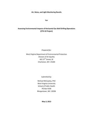
47. 40
Figure 4.1j. Noise levels for Sites A, C, D at Donna Pad. Hours 0, 24, 48 etc. are midnight. Heavy, vertical
lines are noon for each day.
0
20
40
60
80
0 24 48 72 96 120 144 168 192 216 240 264
Sound Level (dBA)
Time (Hours)
Site A
0
20
40
60
80
0 24 48 72 96 120 144 168 192 216 240 264
Sound Level (dBA)
Time (Hours)
Site C
0
10
20
30
40
50
60
70
0 24 48 72 96 120 144 168 192 216 240 264
Sound Level (dBA)
Time (Hours)
Site D

48. 41
4.1.9 SO2 Results
Data for SO2 are available for the entire monitoring period, July 21‐August 1 (Figure 4.1k). The average
concentration of SO2 at the Donna pad was 3.3ppb, with peaks not exceeding 23ppb. Calculating 1‐
hour averages from the one‐minute data for a more direct comparison with the NAAQS for SO2 results in
a range of 1‐hour averages of 1.4ppb – 11.5ppb. Similarly, calculating 3‐hour averages from the one‐
minute data results in a range of 1.9ppb –10.4ppb.
Figure 4.1k. One‐minute average SO2 concentrations .

49. 42
4.2 Weekley Pad (Flowback)
The laboratory was moved from the Donna pad site to the Weekley pad site near New
Martinsville, WV in western Wetzel County on August 2, 2012. The laboratory was located
approximately 200m southwest of the well pad in the yard of a nearby resident with
coordinates of 39°35'24.94"N, 80°46'44.41"W. The resident’s electric service was used to
power the laboratory, so the impact of diesel generator emissions does not need to be
considered for this location. After unpacking, installing, and calibrating, all instruments were
fully operational and collecting data on August 3. Monitoring at this site ended on August 16,
2012. Figure 3 shows a wind rose and histogram for the wind direction and speed during
monitoring at the Weekley pad location. Wind speed was typically very low, with calm
conditions 82% of the time. When there was wind, it was most frequently blowing from the
southwest. At almost all times the laboratory was either monitoring during stagnant conditions
or was upwind of the well pad. Figures for other measured meteorological parameters
(temperature, relative humidity, rainfall, and solar intensity) are included in Appendix C.

50. 43
Figure 4.2a. Wind rose and histogram for wind direction and speed during monitoring at the Weekley
Pad.

51. 44
Figure 4.2b. Satellite photo of Weekley pad showing sampling sites (A,B,C) as red dots and location of
DOE trailer as yellow dot. Black circle is the 625 foot setback distance.

52. 45
Figure 4.2c Terrain map of Weekley pad showing sampling sites (A,B,C) as red dots and location of DOE
trailer as yellow dot. Black circle is the 625 foot setback distance.
4.2.1 HC Results
At the Weekley pad site, there were a total of 274 samples. The analyzer ran continuously from
August 3‐16, with a break in the data for several hours on August 9 for a scheduled
preventative maintenance check by a Perkin Elmer technician.

53. 46
Table 4.2. GC‐FID results
4.2.2 Summa Canister HC Results
Only results above the reporting limit (Rpt Limit), that is, the concentration detectable with a
statistical certainty are reported.
Compound Average (ppb) Standard
Deviation
(ppb)
Minimum
(ppb)
Maximum
(ppb)
Frequency of
Detection (%)
Hexane 6.2 23.9 0.0 375.8 54
Methylcyclopentane 0.4 1.8 0.0 28.1 15
Cyclohexane 0.6 2.5 0.0 36.3 23
2‐methylhexane 1.1 4.5 0.0 65.7 23
3‐methylhexane 1.1 4.4 0.0 62.1 24
n‐heptane 2.3 7.4 0.0 97.9 30
Methylcyclohexane 1.4 4.0 0.0 52.1 30
Toluene 0.7 1.3 0.0 12.1 32
2‐methylheptane 0.4 1.5 0.0 15.5 16
3‐methylheptane 0.5 1.9 0.0 19.9 17
n‐octane 1.0 3.0 0.0 27.6 22
Nonane 0.4 1.4 0.0 11.5 12
Ethane 75.9 199.9 3.3 3,169 100
Propane 71.9 285.1 2.1 4.639 100
Isobutane 20.8 73.3 0.0 1,158 97
n‐butane 44.5 199.9 1.0 3,249 100
Isopentane 17.0 24.0 0.0 186 100
n‐pentane 19.2 75.6 0.0 1,212 99
2,3‐dimethylbutane 0.4 2.3 0.0 35.3 11
2‐methylpentane 4.7 15.2 0.0 240 76
3‐methylpentane 3.0 9.7 0.0 151 67
Isoprene 6.6 5.2 0.0 23.8 90

54. 47

55. 48

56. 49

57. 50
4.2.2.1 PID Results
Figure 4.2.2a. Results for Site C for 8/7‐13/2012.
Instrument malfunctions occurred at sites A and B resulting in loss of data for those sites for the
PID.
4.2.3 Ozone Results
Ozone data are available for the entire monitoring period at this site, August 3‐16 (Figure 4.2d).
The average ozone concentration using one minute data at the Weekley pad was 30ppb, and
the maximum hourly average concentration was 91ppb. Day‐to‐night variations ranged from
20‐85ppb. Calculating 8‐hour averages to more directly compare to the NAAQS results in a
range of 8‐hour averages of 4ppb – 78ppb.
0
2
4
6
8
10
12
14
16
18
20
0 1 2 3 4 5 6 7
Hydrocarbon Concentration (ppb)
TIME (days)

58. 51
Figure 4.2d. One‐minute average ozone concentrations at the Weekley pad.
4.2.4 NOx Results
Data for NOx are available for the entire monitoring period at the Weekley pad site, August 3‐16
(Figure 4.2e). The average of the one‐minute NOx concentration measurements was 3.4ppb,
with an hourly average maximum of 12ppb.