SlideShare ist ein Scribd-Unternehmen logo
1 von 60
Downloaden Sie, um offline zu lesen
The outflow of the Boomerang Nebula
The coldest object in the Universe
MSc thesis in Physics and Astronomy
JUSTIN SALÉR-RAMBERG
Department of Earth and Space Sciences
CHALMERS UNIVERSITY OF TECHNOLOGY
Gothenburg, Sweden 2016
Master’s thesis 2016:NN
The outflow of the Boomerang Nebula
The coldest object in the Universe
JUSTIN SALÉR-RAMBERG
Department of Earth and Space Science
Radio Astronomy and Astrophysics
Chalmers University of Technology
Gothenburg, Sweden 2016
The outflow of the Boomerang Nebula
The coldest object in the Universe
JUSTIN SALÉR-RAMBERG
© JUSTIN SALÉR-RAMBERG, 2016.
Supervisors: Wouter Vlemmings and Theo Khouri, Department of Earth and Space
Sciences
Examiner: Wouter Vlemmings, Department of Earth and Space Sciences
Master’s Thesis 2016:NN
Department of Earth and Space Sciences
Radio Astronomy and Astrophysics
Chalmers University of Technology
SE-412 96 Gothenburg
Telephone +46 31 772 1000
Cover: An image of the Boomerang Nebula taken by the Hubble Space Telescope
Typeset in LATEX
Printed by [Name of printing company]
Gothenburg, Sweden 2016
iv
The Outflow of the Boomerang Nebula
The coldest object in the Universe
JUSTIN SALÉR-RAMBERG
Department of Earth and Space Sciences
Chalmers University of Technology
Abstract
The Boomerang Nebula is a preplanetary nebula with a massive and fast outflow.
The gas in the outflow is seen as absorption against the cosmic microwave back-
ground, making it the coldest known naturally occurring object in the Universe.
Like an interstellar refrigerator, the outflow cools itself adiabatically. Old obser-
vations with Swedish-ESO Submillimetre Telescope (SEST) were consistent with a
constant-velocity outflow, but more recent observations, with Atacama Large Mil-
limeter/submillimeter Array (ALMA), pointed to a model with an outflow velocity
which varies radially. This thesis aims to reproduce the ALMA observations by
considering two different scenarios, a scenario with an explosive event in which the
material was ejected with a range of velocities and a scenario with an outflow with
a time variable expansion velocity. The best-fit models for both scenarios produce
similar spectra on the large scale, as the Boomerang Nebula in a larger region, but
have difficulties matching the spectra along the line of sight through the center of
the shell. The models that fit the data the best are similar too each other. The
thesis also shows a model with a larger shell size than observed, that provides a
good fit to the observations. While it is outside the scope of this thesis, it serves as
a clue for future analysis of the Boomerang Nebula.
Keywords: Stellar Physics, Astronomy, Stellar Winds, Outflow, Preplanetary Neb-
ula
v
Acknowledgements
First of all, I want to thank my supervisors Wouter Vlemmings and Theo Khouri
who have dedicated a lot of time and effort to guide me along my thesis. They
have had to answer to a lot of stupid questions and listen to a lot of stupid ideas. I
want to thank them for not giving up and kept supporting me until the very end.
Without their unwavering support this thesis would not have been possible. I want
to thank the rest of the Star Formation and Evolved Star group for welcoming me
into their circle and teaching me a lot about the field.
I want to thank Ivan Marti-Vidal for a crash course in CASA python scripts. I want
to thank the rest of the staff at Onsala Space Observatory for being among the most
friendly, curious and dedicated people I have ever had the chance to meet. I am
really grateful for the chance to spend half a year with you. I also want to thank
my family for always supporting me. And most of all I want to thank my other half,
Wenzhao Liu, for forcing me to work and helping me to relax. Justin
Salér-Ramberg, Gothenburg, August 2016
vii
Contents
1 Introduction 1
1.1 Units . . . . . . . . . . . . . . . . . . . . . . . . . . . . . . . . . . . . 2
1.2 Star formation and the main sequence . . . . . . . . . . . . . . . . . 3
1.3 Red giant branch and asymptotic giant branch . . . . . . . . . . . . . 5
1.4 Planetary nebulae . . . . . . . . . . . . . . . . . . . . . . . . . . . . . 5
1.5 Stellar effects on the ISM . . . . . . . . . . . . . . . . . . . . . . . . . 6
1.6 Boomerang Nebula . . . . . . . . . . . . . . . . . . . . . . . . . . . . 7
1.7 Probing the circumstellar environment . . . . . . . . . . . . . . . . . 8
1.8 Telescopes . . . . . . . . . . . . . . . . . . . . . . . . . . . . . . . . . 10
2 Stellar Winds 11
2.1 Heating and cooling processes . . . . . . . . . . . . . . . . . . . . . . 12
2.2 Photodissociation . . . . . . . . . . . . . . . . . . . . . . . . . . . . . 13
3 Motivation and methods 15
3.1 Outflow simulations . . . . . . . . . . . . . . . . . . . . . . . . . . . . 18
3.1.1 Explosion scenario . . . . . . . . . . . . . . . . . . . . . . . . 18
3.1.2 Decreasing velocity scenario . . . . . . . . . . . . . . . . . . . 19
3.1.3 Temperature profile . . . . . . . . . . . . . . . . . . . . . . . . 19
3.2 Radiative transfer . . . . . . . . . . . . . . . . . . . . . . . . . . . . . 19
4 Results 23
4.1 Explosion scenario . . . . . . . . . . . . . . . . . . . . . . . . . . . . 24
4.2 Decreasing velocity scenario . . . . . . . . . . . . . . . . . . . . . . . 31
4.3 Considering a large shell size . . . . . . . . . . . . . . . . . . . . . . . 34
5 Conclusion 39
5.1 Interpretation of Results . . . . . . . . . . . . . . . . . . . . . . . . . 39
5.2 Wind mechanism . . . . . . . . . . . . . . . . . . . . . . . . . . . . . 39
6 Future Prospects 43
Bibliography 45
ix
Contents
x
List of Figures
1.1 A Hertzsprung Russel diagram showing the relationship between the
luminosity and the temperature of a star. This plot clearly shows the
main sequence full of young stars. The central star of the Boomerang
Nebula is a post-AGB star. It has just left the AGB branch and is
on it’s way to become a white dwarf. [1] . . . . . . . . . . . . . . . . 4
1.2 A schematic view of the AGB star during thermal pulses. Hydrogen
burning happens in the envelope of the star producing helium. When
enough helium has been created, helium burning is reignited pushing
out the hydrogen envelope. . . . . . . . . . . . . . . . . . . . . . . . . 6
1.3 A schematic view of the Boomerang Nebula and its shell. The focus
of this thesis is the Nebula’s absorbing outer shell, the coldest known
naturally occurring object in the Universe. . . . . . . . . . . . . . . . 8
3.1 The spectra of the CO(J = 1 − 0) line from the SEST+ALMA data,
given at four different apertures. The spectrum in the upper-left
panel is similar to the SEST spectrum, while the spectrum in the
lower-right panel was obtained from a much smaller aperture. . . . . 16
3.2 The first upper-left panel shows the CO(J = 1 − 0) line from a large
aperture around the Boomerang Nebula. It is included to show how
the original SEST data looked like. From the spectrum, it is hard
to say anything about the velocity’s radial behavior. In the center of
the line, there is emission from the inner shell. The upper-right panel
shows the same line for a constant velocity model, to show that it is
possible to describe the SEST data with it. The lower-left panel shows
the CO line extracted from the ALMA data using an aperture smaller
than the shell. The lower-right panel shows how a constant velocity
model would look in the same aperture. A constant velocity model is
not able to describe the ALMA spectrum and, hence, a model with a
radially dependent velocity profile is required. . . . . . . . . . . . . . 17
3.3 How the simulation determined if two mass bins collided. The parti-
cles had positions ri and rj and velocities υi and υj respectively. . . . 18
4.1 The logarithm of the density for an explosion model. The explosion
used the parameters υc = 120km/s and υo = 100 km/s (see Equation
(3.3)). The total gas mass is M = 2.9M . The model includes an
AGB wind moving at a velocity of 15 km/s and has a mass loss rate
of ˙M ≈ 10−5
M /year. . . . . . . . . . . . . . . . . . . . . . . . . . . 24
xi
List of Figures
4.2 The temperature profile for an explosive wind colliding with an AGB
wind. Th explosion uses the parameters υc = 120km/s and υo = 100
km/s (see Equation (3.3)) and the total gas mass is 1.4M . The
AGB wind has a velocity at 15 km/s and a mass loss rate rate of
˙M ≈ 10−5
M /year. . . . . . . . . . . . . . . . . . . . . . . . . . . . . 25
4.3 Spectra for an explosion scenario model with an AGB wind, at differ-
ent times. The explosion model has parameters υc = 120 km/s and
υo = 100 km/s (see Equation (3.3)) and a total mass of 2.9 M . The
AGB wind is moving at a constant velocity of 15 km/s and had a
mass loss rate of 10−5
M /year. After 1150 years, the AGB wind has
left the shell. . . . . . . . . . . . . . . . . . . . . . . . . . . . . . . . 25
4.4 The Gaussian distribution of an explosion with υc = 120 km/s and
υo = 40 km/s. The velocity at the outer edge of the cold shell is
υout = υc +2υo and the velocity at it’s inner edge is υin. At this time,
most of the mass from the explosion is inside the shell. . . . . . . . . 26
4.5 The density profile for different parameters in the explosion scenario.
The time is chosen accordingly to Equation (4.1). The profiles are
compared to ρ ∝ r−2
, the density profile for a constant wind velocity. 27
4.6 The temperature profile for different velocity parameters, υo and υc,
in the explosion model. The time is chosen accordingly to Equation
(4.1). The temperature asymptotes T ∝ r−4/3
, the case of constant
velocity without molecular heating, as the outflow velocity increases
and the photoelectric heating weakens. . . . . . . . . . . . . . . . . . 27
4.7 The absolute value of the different heating and cooling mechanisms
in the explosion scenario, 1040 years after the initial explosion. The
parameters υc = 100 km/s and υo = 60 km/s, see Equation (3.3).The
total gas mass in the explosion is 1.4M . . . . . . . . . . . . . . . . . 28
4.8 The intensity map of an outflow with the explosion scenario, 1150
years after the initial explosion. The parameters υc = 220 km/s and
υo = 120km/s, see Equation (3.3).The total gas mass in the explosion
is 2.9M . The color map is for velocities at υ = 0.5 km/s . . . . . . 28
4.9 Spectra from the explosion scenario, for different values of υc. The
total gas mass is M = 2.9M . The offset velocity is υo = 100 km/s. . 29
4.10 Spectra from the explosion scenario for different values of υc. The
total gas mass is M = 2.9M . The offset velocity is υo = 40 km/s. . . 29
4.11 Spectra from the explosion scenario for different values of υo. The
total gas mass is M = 2.9M . The central velocity is υc = 120 km/s. 30
4.12 Spectra from the explosion scenario for different gas mass M. The
central velocity is υc = 120 km/s and the offset velocity is υo = 100
km/s. . . . . . . . . . . . . . . . . . . . . . . . . . . . . . . . . . . . 30
4.13 The best fit of the explosion scenario to the SEST+ALMA data. This
model has υc = 120 km/s, υo = 100 km/s and M = 1.8M . . . . . . . 30
4.14 The radial velocity profile for different ejection velocity parameters,
vi and α. As α increases, the velocity profile becomes linear. . . . . . 32
4.15 The radial density profile for different ejection velocity parameters,
vi and α. The density is much steeper than a constant velocity model. 32
xii
List of Figures
4.16 The radial temperature profile for different ejection velocity param-
eters, vi and α. The temperature approaches T ∝ r−4/3
, when υi
increases, which is the case of a constant velocity and no heating. . . 33
4.17 The absolute value of the heating and cooling mechanisms in the
decreasing model, with t = 1388 years and υ(r = 0, t) = 165 ∗ t−0.5
km/s. The dominant heating factor is the photoelectric heating, just
weaker than the adiabatic cooling. . . . . . . . . . . . . . . . . . . . . 33
4.18 The spectra of υ(r = 0, t) = 165(t/year)−α
km/s, where α is varied
between 0.1 and 1. The spectra are taken when the front of the gas
reaches the outer edge of the outer shell. . . . . . . . . . . . . . . . . 34
4.19 The spectra of υ(r = 0) = υi(t/year)−0.8
, where υi is varied. The
spectra are taken when the front of the gas reaches the outer edge of
the outer shell. . . . . . . . . . . . . . . . . . . . . . . . . . . . . . . 35
4.20 The spectra of υ(r = 0) = 200(t/year)−0.8
km/s, where the shell mass
is varied. The spectra are taken when the front of the gas reaches the
outer edge of the outer shell. . . . . . . . . . . . . . . . . . . . . . . . 35
4.21 The best fit for the decreasing wind scenario to the SEST+ALMA
data. The ejection velocity is υ(r = 0) = 200(t/year)−0.8
km/s and a
shell mass 2.97M . . . . . . . . . . . . . . . . . . . . . . . . . . . . . 36
4.22 The fit of an explosion model where the outer shell has a radius 75 .
The velocity parameters are vc = 160 km/s and vo = 60 km/s. The
total gas mass in the ejection is 2.9M . . . . . . . . . . . . . . . . . . 37
5.1 The spectra from the two scenarios’ best models. The explosion model
was ejected instantly with a Gaussian velocity distribution with the
central velocity, vc = 100 km/s and the velocity offset, vo = 60 km/s.
The total mass in the explosion was 1.4M . The time decrease model
used an ejection velocity v(r = 0, t) = 200(t/year)(
− 0.8) and a shell
mass 2.97M . . . . . . . . . . . . . . . . . . . . . . . . . . . . . . . . 40
5.2 The velocity, density and temperature profiles from the two scenarios’
best models. The explosion model was ejected instantly with a Gaus-
sian velocity distribution with the central velocity, vc = 100 km/s
and the velocity offset, vo = 60 km/s. The total mass in the explo-
sion was 1.4M . The time decrease model used an ejection velocity
v(r = 0, t) = 200(t/year)(
− 0.8) and a shell mass 2.97M . . . . . . . 40
xiii
List of Figures
xiv
1
Introduction
Stars are massive interstellar nuclear reactors in which new elements are created [1].
Without the stars there would not be any heavy elements. " We are all made of
stardust " is an often repeated quote. Without the processes that occur in the stars,
the giant element factories in the sky, there would be no Earth and there would not
be any humans. The stars have an important role in the Universe and for life. That
makes it very important to study them.
More than 400 years have passed since Giordano Bruno realized that the stars and
the Sun were the same type of entity [1]. He was the first to propose that stars, just
like the Sun, have their own planets and other objects orbiting them. There was an
easy way to learn more about stars right in our back alley, by investigating our own
star, the Sun.
In the last 400 years our understanding has increased vastly and recently more
advanced telescopes and computers have made it easier for astronomers to study
the stars. Nonetheless, there are still gaps to be filled by avid researchers. A lot is
known about Sun-like stars, but exotic objects are often poorly understood. With
more accurate telescopes distinct behaviors can be revealed, hidden in previous
observations.
Stars, just like living beings, evolve through several phases [1]. A star spends most
of its lifetime on what is called the main sequence, in hydrostatic equilibrium. Hy-
drostatic equilibrium implies that the nuclear fusion inside the star counterbalances
the gravitational forces, preventing the star from imploding. When the nuclear fuel
has been depleted within the core, the stellar structure readjusts to maintain the
equilibrium. Stars with masses close to our Sun grows into giant stars with high
mass loss rates [2]. After the star has ejected most of its material, the remnants
of the central star can ionize it. With old telescopes, the ionized envelope looked
similar to giant gas planets and is earning them the name "planetary nebula".
The target of this thesis is the Boomerang Nebula which is a preplanetary nebula.
In Preplanetary nebulae the outflow has not yet been ionized [3]. Compared to other
preplanetary nebulae, the Boomerang Nebula holds several distinguishing features
that separate it from its kin. Its rarest feature is its outflow which is the coldest
known naturally occurring medium in the Universe [4].
The Boomerang Nebula was first observed in detail by Sahai and Nyman 1995 [4]. To
fit the observations, they constructed a model with an assumption that the outflow
had a constant velocity in the cold region. However new measurements from 2013
showed a multitude of velocities [5]. The velocity of the outflow had to have a radial
dependence. The main goal of this thesis is to obtain a deeper understanding of the
radial dependence of the outflow velocity. By understanding the behavior of unique
1
1. Introduction
objects such as the Boomerang Nebula, we will improve our understanding of the
late phases of stellar evolution.
The first chapter is an introduction chapter, which gives a quantitative description
and introduces the reader to the subject. It covers the units that are used in as-
tronomy, as well as a short tour of stellar evolution. The third chapter’s focus is
stellar wind models and how they can be used to describe the Boomerang Nebula’s
outflow. The fourth chapter contains the motivation to this thesis and a description
of the methods. The fifth chapter shows the result of the modelling and comparisons
with observations. In the sixth chapter the results are discussed. The seventh and
final chapter gives an outlook on future uses of the work in this thesis. It also covers
potential upgrades to the models and the next steps necessary to understand the
Boomerang Nebula.
1.1 Units
It is no longer convenient to use standard SI units when working with the large
scales in astronomy. While a meter or a kilogram works great when dealing with
every day life, larger units are required when working with the large scales of the
Universe.
For example, astronomers count mass in solar masses, M [1]. A solar mass is
M = 1.989 × 1030
kg. (1.1)
The lifetime of a star is in scales of millions or billions of years, so during a second
only an insignificant amount of mass is lost. The commonly used unit used for
mass-loss rate of stars is M /year [1], where
1M /year = 6.305 × 10²²
kg/s. (1.2)
The movement of stellar objects tends to be estimated in kilometers per second.
Giant stars can eject material moving at 500 km/s. Comparatively the speed of a
bullet is 1 km/s. And while a bullet hits a wall within a few seconds, the ejected
material moves freely. During a year, a short time compared to the stellar lifetimes,
the ejected material travels 2 × 10¹⁰
km. During the same time starlight travels
9 × 10¹²
km. These distances, which normally would seem immense, are quite small
in the Universe. Measuring the large distances light and matter travel in space
requires much larger units than measuring distances on Earth.
Different units are chosen based on context. For describing the close environment
of a stellar object, the common choice is astronomical units (AU), where
1 AU = 1.496 × 10¹¹
m. (1.3)
1 AU is the distance between the Earth and the Sun, or more explicitly since the
Earth’s orbit around the Sun is elliptical, it is defined as the average of the minimum
and maximum distance between them [1]. Initially this distance was calculated using
the parallax method, which is still used to calculate the distance to stars.
The parallax method uses the angle between a near object and a distant object
[1]. When the observer moves, the nearer object seems to move with respect to the
2
1. Introduction
farther away one. With the distant object as a reference point, the change in the
angle between the two points can be noted. The parallax angle, p, is defined as half
this change in angle, and with triangulation the distance to the nearby object is
D =
d
tan(p)
, (1.4)
where d is half the distance between the observation points.
The distance to other stars is so large that the parallax between two locations on
earth is too small to be measured accurately. Instead the parallax angle is observed
with a six month interval. In this time the Earth has travelled halfway around the
Sun so that d = 1 AU. This distance is many magnitude larger than the Earth
radius giving much more accurate results.
But even when using the orbit of the earth, the parallax angle is still very small.
Instead of degrees, astronomers use arc minutes and arc seconds for the parallax
angle.
An arc minute, or 1 , is defined as one sixtieth of a degree and similarly an arc
second, or 1 , is one sixtieth arc minute. The unit for the distance to stars is
1 parsec =
1 AU
tan(1 )
= 3.086 × 10¹⁶
m, (1.5)
These units are necessary to know for reading astronomy papers, but more important
to understand are the processes in the Galaxy. Next follows an introduction of the
creation of the stars and their impact on the Galaxy.
1.2 Star formation and the main sequence
Our galaxy is not only stars and empty space. The medium between the stars, called
the interstellar medium (ISM), contains gas and dust [6]. 91% of the gas atoms in
the ISM are hydrogen. The second most prevalent element in the ISM is helium,
accounting for most of the remaining 9%. The relationship between stars and the
gas is cyclical, the stars are born from the gas and during their lifetime the stars
push it back into space.
More specifically, stars are born within giant molecular clouds (GMCs). GMCs are
humongous clouds of molecular gas, with diameters up too 100 parsec [7]. Just
like stars, the GMCs are in hydrostatic equilibrium [6]. But eventually instabilities
within the cloud lead to the collapse of pockets of gas. The molecular gas from
the GMC is condensed in a few dense cores. At the center of each core a protostar
forms.
The accreted material have small rotational velocities which, to preserve the angular
momentum, cause the cores to spin faster and faster. Like a pizza, the cores flatten
and form a preplanetary disc around the protostar. The protostar starts ejecting
matter perpendicular to its rotation. As the preplanetary disc spins, the dust in the
disc combines into larger and larger grains of dust. After millions of years, most of
the dust has bundled together into planets and other objects such as asteroids.
In the protostar, the compression due to gravity leads to an increase in density,
temperature and pressure. When the pressure is high enough to counterbalance
3
1. Introduction
Figure 1.1: A Hertzsprung Russel diagram showing the relationship between the
luminosity and the temperature of a star. This plot clearly shows the main sequence
full of young stars. The central star of the Boomerang Nebula is a post-AGB star.
It has just left the AGB branch and is on it’s way to become a white dwarf. [1]
the gravity the cloud regains hydrostatic equilibrium. The collapse stops, but the
protostar is too cold for nuclear fusion.
At a temperature of around 2000 K , the thermal energy causes the molecular
hydrogen inside the nucleus of the core to dissociate [8]. Soon after, the hydrogen
and the helium are ionized, and at 107
K, the Star’s nucleosynthesis can start [9].
At the protostar’s nucleus the hydrogen atoms fuse into helium, releasing energy.
Since this process is exothermic, it is called hydrogen burning.
When the hydrogen burning starts the protostar has transformed into a star. The
newborn star is located on the main sequence, where it will spend 90 % of its
lifetime [1]. Stars in the main sequence are in hydrostatic and thermal equilibrium.
Thermal equilibrium states that the energy generation of the star is balanced by
it’s luminosity. The correlation between stars in the main sequence can be seen
in a Hertzsprung-Russel (HR) diagram (see Figure 1.1). The HR diagram shows
the relationship between the luminosity and the effective temperature of the stars.
Depending on a star’s position on the HR diagram its evolutionary phase can be
inferred.
4
1. Introduction
When the nucleus of a main sequence star is depleted of hydrogen, it is impossible
for hydrogen burning to continue within it [3]. With no hydrogen burning, there is
no pressure to balance out the gravity. This causes the nucleus to lose hydrostatic
equilibrium and collapse. The gravitational energy is converted into thermal energy,
increasing the temperature and triggering hydrogen burning in a shell around the
core. The helium produced in the shell falls back into the core, increasing the core’s
density and temperature.
1.3 Red giant branch and asymptotic giant branch
The higher temperature enables higher rates of hydrogen burning in the shell than
earlier within the nucleus. The increase in energy output causes the star to expand
to several magnitudes bigger than its main sequence size. As the surface area of the
star increases the surface temperature decreases. The nucleus is hot and massive,
while the star has a low effective temperature and a critically low density. Due to
the color and the size of the star, it is labeled as a red giant. Red giants are located
on the red giant branch (RGB) in the HR diagram (Figure 1.1).
When the nucleus has reached a temperature of 108
K the helium fuses into beryllium
[3]. Through fusing with other helium atoms, it forms carbon and then oxygen. Dur-
ing this process, called helium burning, the star’s effective temperature is increasing
with conserved luminosity. The star simultaneously burns helium in its nucleus and
hydrogen in a shell. After this phase, called the horizontal branch (HB), the star
enters the asymptotic giant branch (AGB).
During the HB, the nucleus expends its helium [3]. Left in the nucleus is carbon and
oxygen, with too low temperature for them to fuse. Instead helium burning starts
in a shell around the nucleus. The star is again a red giant. The AGB is said to be
asymptotic since it approaches the RGB asymptotically in the HR diagram.
After the helium shell is depleted, the star derives its energy from hydrogen burn-
ing in a thin hydrogen shell [2]. The helium produced forms a thin layer of helium
between the hydrogen shell and the nucleus. When enough helium has been accumu-
lated, helium burning is reignited. The helium burning will push out the hydrogen
shell and extinguish the burning there. This process is referred to as a thermal pulse.
After the thermal pulse, hydrogen burning is reignited in the the shell accumulating
more helium for another thermal pulse (see Figure 1.2). Thermal pulses increase the
luminosity and size of the star periodically. During the pulses, and to a lesser extent
during the entire AGB phase, a lot of mass is ejected into the star’s circumstellar
environment.
1.4 Planetary nebulae
When an AGB star has ejected almost all of its hydrogen envelope, it will enter the
preplanetary nebula (PPN) phase [2]. When looking at PPNs, the focus does not lie
on the central star, but instead on the ejected material. This is because the ejected
gas can be many times the mass of the star.
5
1. Introduction
Figure 1.2: A schematic view of the AGB star during thermal pulses. Hydrogen
burning happens in the envelope of the star producing helium. When enough helium
has been created, helium burning is reignited pushing out the hydrogen envelope.
During the PPN phase, the central star is too cold to ionize the ejected material.
Preplanetary nebulae are said to be reflection nebulae. Reflection nebulae have very
little emission in the visible spectra and were originally detected by the scattering
of the light from their central stars.
From the hydrogen burning in the shell, the star’s effective temperature is increasing.
When the central star has become hot enough to produce ultraviolet light, it ionizes
the ejected envelope. The ionized envelope becomes an emission nebula, showing an
appearance similar to giant gas planets such as Jupiter.
The star has entered the planetary nebula (PN) phase. The PN phase is the star’s
last high-luminosity phase. When the hydrogen shell exhausts, the central star
becomes too cold to ionize its increasingly distant gas cloud and become a white
dwarf. White dwarfs are dense stars, with no internal source of energy. Meanwhile
the gas cloud turns invisible, ending the planetary nebula phase.
Planetary nebulae comes in various shapes [10]. Everything from bipolar and disc-
shaped to quadripolar and point-symmetric planetary nebulae have been observed.
The morphology of the planetary nebulae is highly dependent by how it acts during
the PPN phase. One of the reasons to study the Boomerang Nebula is to understand
how the shaping of PN takes place.
1.5 Stellar effects on the ISM
While most stars enter the RGB after depleting hydrogen in their nuclei, not all of
them do. Main sequence stars with a mass below 0.5 M never become hot enough
to initiate helium burning. Instead they cool down and turn into white dwarfs [1].
Stars with high mass also have unique features, main sequence stars heavier than
6
1. Introduction
2 M smoothly proceeds with helium burning after the hydrogen is depleted. They
then have helium burning and hydrogen burning in their shell simultaneously. Stars
with a main sequence mass above 8M are able to burn the carbon within its core to
produce magnesium [2]. Heavier elements are produced in supergiants , stars with
main sequence masses above 10M , named as they grow much larger than other
stars [11]. Super giants are composed of several shells, each with different elements
burning, and eventually build up an iron nucleus [12].
When a super giant depletes its fuel, it collapses into a supernova. Supernovae are
titanic explosions able to outshine entire galaxies [1]. The total radiant energy of
a supernovae is the same as our Sun will produce during its entire life. The high
energy of supernovae make them the most energetic nuclear reactors in the Universe.
Most natural elements heavier than iron are produced in supernovae. The exception
is specific elements created through slow neutron capture processes in AGB stars’
shell.
From the chemical composition of the ISM it is possible to learn about nearby stars.
While most helium and hydrogen were created in the Big Bang, heavier elements
are often created in stars [1]. And generally, the heavier an element is, the bigger
was the nuclear reactor it was produced in.
It is not only gas that the stars eject into ISM, but also dust. Most of the cosmic
dust in the ISM is formed in AGB stars or supernovae [2]. Just like the gas can
be traced to its progenitors, so can the dust. Stars with more oxygen than carbon
produce oxygen rich dust, oxides and silicates, and stars with more carbon produce
carbon rich dust, carbocaneous dust. Supernovae have both carbon rich and oxygen
rich layers and therefore can produce both kind of dust. But since most of the layers
are oxygen rich, the dust from supernovae are dominantly silicates. All AGB stars
are initially oxygen rich, But AGB stars with a mass between ≈ 1.6M to 4M will
become carbon rich. Therefore, the surrounding dust contain information about the
chemical structure of the stars, as well as limits to an AGB star’s mass.
1.6 Boomerang Nebula
The Boomerang Nebula is a biconal preplanetary nebula, discovered by Wegner and
Glass in 1979 [13]. Its most unique feature is its outflow, which is the coldest known
natural occurring object in the entire Universe [4]. As a remnant of the Big Bang,
the Universe is coated with Cosmic Microwave Background Radiation (CMBR),
with a characteristic temperature around 2.7 K. Normally the CMBR has to be
treated as noise, as the emission from stars towers about it, but the Boomerang
Nebula’s outflow is cold enough to absorb the photons emitted from the CMBR. By
absorbing the CMBR photons, the outflow is self-shielded and the CMBR photons
can not penetrate and heat the innermost regions.
Another interesting aspect of the Boomerang Nebula, and bipolar nebulae in general,
is that the outflow seems to carry a much larger amount of linear momentum than
expected from the current model for radiation-pressure-driven outflows in evolved
stars. The mechanism behind the driving of these winds is not understood and is
one of the reasons for studying these enigmatic objects [14].
7
1. Introduction
Figure 1.3: A schematic view of the Boomerang Nebula and its shell. The focus
of this thesis is the Nebula’s absorbing outer shell, the coldest known naturally
occurring object in the Universe.
The outflow of the Boomerang Nebula is separated in two distinct shells [4], illus-
trated in Figure 1.3. The inner shell is biconal, with a temperature slightly above
the CMBR and a velocity around 35 km/s. It is located between 2.5 (3743 AU)
and 6 (8690 AU) from the central star. The outer shell, which is colder than the
CMBR, is located between 6 (8690 AU) and 33 (48129 AU). It does not follow
the biconal shape of the inside and is instead almost spherical. The outer shell has
a multitudes of velocities, peaking at around 165 km/s.
In the outflow, the hydrogen has returned to its molecular state. Even if hydrogen
is the most dominant element in the molecular gas, molecular hydrogen has no
permanent dipole moment [6]. It radiates very poorly at radio wavelengths, making
it difficult to detect. Due to this, other molecules are used to trace the outflow. A
good tracer is carbon monoxide (CO). CO has stable bonds and several emissions
in the radio spectrum.
1.7 Probing the circumstellar environment
When a molecule changes state, it absorbs or emits a photon [15]. These photons,
detectable with telescopes, give us information about distant objects. The energy
levels, or states, of the molecules are quantized so that when a molecule absorbs or
emits a photon, its frequency and energy can be related to a state transition.
Molecules have three different kinds of state transitions [15]. The most energetic
transitions are electronical. These transitions happen when the electrons inside
the molecules are excited or deexcited, emitting UV photons. The second most
energetic are the vibrational transitions. When the molecules transit between vi-
brational states they emit infrared (IR) photons. The least energetic transitions of
the molecules are the rotational transitions. The rotational transitions emit photons
in the radio, sub-millimeter and IR wavelengths. Radio photons can be detected on
8
1. Introduction
the Earth’s surface, while UV and IR photons are blocked by the atmosphere. Due
to this, the rotational transitions are often the ones that can be observed in the
greatest detail.
Rotational transitions can be modelled as a rigid rotor [1]. In classical physics the
energy of a rigid rotor is Erot = L2
2I
, where L is the angular momentum and I is the
rotor’s moment of inertia. Similarly the energy of the rotation states are
E(J) =
J(J + 1)h2
8π2I
= B0J(J + 1). (1.6)
In this equation, J is the quantum number for the rotational states, with J = 0
being the rotational ground state. Linear molecules, like CO, follows the rotational
transition rule, ∆J ± 1. The constant, h, in the equation is Planck’s constant. The
energy of a photon that is emitted from J → J − 1 is
Ephoton = ∆E(J) = E(J) − E(J − 1) = B0(J(J + 1) − J(J − 1)) = 2B0J. (1.7)
For example, CO has the rotational constant B0 = 0.238 meV [6]. Equation (1.7)
then states that the rotational transition CO(J = 1 → 0) emits a photon with an
energy of 0.476 meV. From Planck’s relation the frequency of the photon is 115.27
GHz. Planck’s relation correlates the energy, Ephoton with the frequency, ν as
Ephoton = hν. (1.8)
The emission lines can be used to obtain the target’s minimum temperature [6].
The thermal energy of an object is given as Et = kBT, where kB is the Boltzmann
constant and T is the target’s temperature. For example, for CO to continually emit
CO(J = 2 → 1), the molecules need to be excited to the second rotational level.
Using Equation (1.6) and B0 = 0.238 meV, T ≥ 6B0
kb
= 16.6 K.
Normally the emission source is moving, so that the frequency will be shifted by the
Doppler effect [1]. The Doppler effect is a relativistic effect. It states that if the
emission source is moving at a velocity, ∆υ, relative to the observer, the observer
sees a photon with frequency
νc = ν0(1 +
∆υ
c
). (1.9)
Here, c, is the speed of light and, ν0, is the emission frequency excluding the Doppler
effect. While it may require more than one emission peak to find ∆υ, the relative
velocity is useful information of the target.
The Doppler effect also has another impact on the emission line. Since the Doppler
shift perceived by an observer is determined by the velocity component along the
line of sight, different regions of a circumstellar envelope expanding with velocity υ
will present different Doppler shifts. A given observed line is said to be broadened by
this effect. The projected velocity changes gradually from −υ for gas in the part of
the envelope moving away from the observer to 0 in the plane of the sky to υ in the
part of the envelope approaching the observer. On top of this, any radial variations
of the expansion velocity may also contribute to the broadening of a given line.
9
1. Introduction
1.8 Telescopes
Measuring the emission lines of stellar objects, thousands of parsecs away, requires
large telescopes with advanced equipments. The angular resolution of a telescope is
inversely proportional to its aperture diameter [16].
This thesis uses data sets obtained with two different telescopes. The first was
obtained in 1997 by Sahai and Nyman with the Swedish-ESO Submillimeter Tele-
scope (SEST) [4]. SEST was a radio telescope in La Silla, Chile, that was active
between 1987 and 2003 [17]. It had an aperture diameter of 15 m and, for the
CO(J = 1 − 0), an angular resolution of 42 . As the Angular resolution was larger
than the Boomerang Nebula (see Figure 1.3), the observation did not provide much
details on the velocity dispersion.
The second data set was obtained in 2013 by Sahai et al. with the Atacama Large
Millimeter/submillimeter Array (ALMA) [5], also located in Chile. ALMA used
an array of 33 telescopes to virtually increase the aperture. In total, ALMA has
55 telescopes [18], moveable to span an aperture with a diameter of 16 km. With
ALMA, it was possible to reduce the angular resolution down to less than 5 , smaller
than the outer shell.
10
2
Stellar Winds
Outflows that originate from stellar atmospheres are called stellar winds [6]. The
focus of this thesis is to model the velocity dependence of the outflow in the outer
shell of the Boomerang Nebula.
Stellar winds collide with gas in the ISM or the circumstellar envelope. These can
usually be distinguished based on differences in parameters such as velocity, density
and temperature. The goal of the wind model is to obtain such parameters for the
Boomerang Nebula’s outflow. They can be obtained from radiative transfer model,
since the emission from the outflow depends on its parameters.
Stellar wind models assume that mass, momentum and energy are conserved [19].
The mass conservation can be modeled by the mass continuity equation
∂ρ(r)
∂t
+ · ρ(r)v(r) = 0. (2.1)
The mass continuity equation has a spatial dependence, using r as the position
vector. At r the density is ρ(r) and the outflow velocity is v(r).
The mass continuity equation can be related to the star’s mass loss ˙M with two
assumptions. The first assumption is spherical symmetry, that the outflow is sym-
metric in all directions from the star. The distance to the center of the star r can
replace r.
The second assumption is that the system is in steady state. This means that the
stellar wind properties are constant in time. Under these assumptions Equation
(2.1) can be rewritten as
˙M = 4πρvr2
. (2.2)
Equation (2.2) is irrelevant for an outflow with a radial dependence, but is useful
for showing relations between parameters in stellar wind models.
The second quantity that is conserved is momentum, for which the conservation
equation is
∂v(r)
∂t
+ v(r) · v(r) = −
P(r)
ρ(r)
−
GM
r2
ˆr. (2.3)
P is the radiation pressure, G is Newton’s gravitational constant and M is the mass
of the star. In the outer shell of the Boomerang Nebula we have a large distance
and a high velocity. Due to this, the contributions from the pressure and gravity
are negligible. Under these assumptions Equation (2.3) can be reduced to
∂v(r)
∂t
+ v(r) · v(r) = 0. (2.4)
11
2. Stellar Winds
This equation can be fulfilled with simple Newtonian mechanics. It is assumed
that the wind can move freely in space without outer constraints. It is simple to
obtain the the radial dependencies of the density and velocity. But to obtain the
radial profiles of the temperature, it is required to consider the heating and cooling
processes in the outflow.
2.1 Heating and cooling processes
The radial dependence of the temperature can be modeled as [20]
dT(r)
dr
= (2 − 2γ)(1 +
r
2v(r)
∂v(r)
∂r
)
T(r)
r
+
γ − 1
nH2 (r)kBv(r)
(H − C). (2.5)
The first term covers the adiabatic cooling. The adiabatic cooling is the dominant
cooling process in the outflow, caused by pressure decrease in a system [21]. The
common gas law states that a decrease in pressure makes it expand. But a system
with neither matter or heat output is adiabatically isolated. When an adiabatically
isolated system expands, it does work on its surrounding, cooling itself. In the
adiabatic cooling term, T is the outflow temperature and γ is the heat capacity
ratio. The heat capacity ratio can be related to the degrees of freedom of the gas,
f,
γ =
f
f + 2
. (2.6)
At T ≤ 300, the rotational excitations of H2, the dominant molecules in the molec-
ular gas, are insignificant. Due to this the molecular gas can be treated as a mono-
atomic gas with f = 3 and γ = 5/3.
The second term in Equation (2.5) contains the molecular heating and cooling pro-
cesses in the outflow. Here nH2 is the number density of the molecular gas, which
is related to the mass density by ρH2 = mH2 nH2 , where mH2 is the mass of a H2
molecule. The constant kB is the Boltzmann constant, relating the system’s thermal
energy and temperature, Et = kBT. Finally H − C is the sum of the heating and
cooling rates.
The dominant heating processes are dust-gas collisional heating, dust-gas adhesion
heating and photoelectric heating [22].
The dust-gas collisional heating [20] comes from gas colliding with dust and is mod-
elled with
Hdg =
3
8
mH2 (nH2 (r))2 Ψ
agρg
v3
drift
1 +
vdrift
v(r)
. (2.7)
The dust properties is the dust-to-gas mass ratio, Ψ, the average dust grain radius,
ag and the average dust grain density, ρg. The model assumed silicate dust with
Ψ = 0.01, ag = 0.1 µm and ρg = 3.3 g/cm3
. Another dust property is the drift
velocity of the dust through the gas, vdrift. This is assumed to be constant at
vdrift = 10 km/s.
The dust adhesion heating [23] can be modelled as
Hdt = 2.008×10⁻³¹
(nH2 (r))2 Ψ
agρg
T(r)(Tdust − T(r)(0.35e
−
Tdust+T (r)
500
+0.1). (2.8)
12
2. Stellar Winds
The expression contains the dust temperature Tdust, which has been assumed to be
constant at 15K. Note that the equation assumes SI units.
The final heating contribution that was considered is the photo-electric heating,
which is the heating of the gas from stray photons. It is covered in
Hpe = KpenH2 (r), (2.9)
where Kpe = 10−33
J/s [24].
The only non-adiabatic cooling term able to affect the temperature is the H2 vibra-
tional line cooling [23],
CH2 = 2.611 × 10⁻³⁴
nH2 (r)(
Tkin
1000
)4.74
. (2.10)
From putting all the heating and cooling factors together in Equation (2.5), the
temperature’s radial dependence can be obtained.
The photoelectric heating came from photons stimulating electronial transitions in
the gas, but if the photons are energetic enough they are able to dissociate the
molecular gas into atoms.
2.2 Photodissociation
At the inner regions of the circumstellar envelope the molecules are shielded by
the gas in the outer region. But in outer regions, the molecular bonds break from
interactions with high energy photons from the ISM. At the so called dissociation
radius, half of the molecules in the gas have dissociated. The dissociation radius
varies between different molecules, relative to their dissociation energy, which is the
minimum energy for a photon to dissociate it [25].
The high dissociation energy of CO is one of the properties that makes it a good
tracer molecule. But even if the dissociation radius of CO is large, it is not infinite.
Outside of its dissociation radius the CO dissociates into C and O atoms. And
although the stellar wind continues, the CO emission or absorption lines dissappear.
13
2. Stellar Winds
14
3
Motivation and methods
The Boomerang Nebula was initially discovered in 1978 by Wegner and Glass [13]. In
1997 its molecular outflow was observed by Sahai and Nyman with SEST (Swedish
ESO Submillimeter Telescope) [4]. They discovered that the nebula’s outflow is
colder than the cosmic microwave background radiation (CMBR). The CMBR is a
remnant from the Big Bang maintaining the Universe’s temperature at 2.7 K. The
outer shell of the Boomerang Nebula (see Figure 1.3) by mimicking the behavior of
a refrigerator. It cools through adiabatic cooling and self-shields from the CMBR.
But the Boomerang Nebula is not only colder than the CMBR, it is also the coldest
known naturally occurring object.
The SEST spectrum of the CO(J = 1 − 0) transition shows absorption in velocities
ranging from roughly −165 km/s to 165 km/s. As explained at the end of Section
1.7, this is caused by Doppler line broadening and reflects the velocity dispersion
in the shell. The SEST spectrum had a beam size of 40 , and resembled the first
plot in Figure 3.1. It shows a wide velocity dispersion that could be explained using
many different models. The emission at the center of the spectrum originates in the
inner shell (see Figure 1.3) and is not considered in the thesis.
Further observations of the Boomerang Nebula were done by Sahai et al. in 2013
with ALMA [5], which used an array of several telescopes to simulate a smaller beam
size. The beam, which was not circular, had a major axis of 4.12 and it’s minor axis
of 1.83 . Figure 3.1 depicts ALMA observations which show that even for smaller
beam sizes, the outer shell shows absorption in a wide range of velocities.
Sahai and Nyman constructed a model with a constant expansion velocity, that could
fit well to the SEST spectrum (see figure 3.2) [4]. However, a constant velocity model
produces two sharp absorption peaks when imaged with a small aperture (see the
last plot in Figure 3.2), in contrast to what is seen in the ALMA observations.
To address this problem, two different scenarios with radially dependent outflow
velocities were considered. The first one is an initial explosion ejecting most of
the gas into the envelope. The second scenario is an outflow with a time-varying
ejection velocity. The scenarios were modelled independently and their parameters
were adjusted to match the ALMA and SEST data.
The outflow was simulated in MATLAB. Assuming spherical symmetry the outflow
could be modelled with one dimensional mass bins. And assuming that the radia-
tion pressure and gravitation had negligible effect, the gas could move freely. The
outflow simulations output the radial profiles of velocity, density and temperature.
The profiles were input into a radiative transfer (RT) model to simulate how light
propagated inside the outflow. The RT model produced the CO(J = 1−0) line that
15
3. Motivation and methods
Figure 3.1: The spectra of the CO(J = 1 − 0) line from the SEST+ALMA data,
given at four different apertures. The spectrum in the upper-left panel is similar to
the SEST spectrum, while the spectrum in the lower-right panel was obtained from
a much smaller aperture.
16
3. Motivation and methods
Figure 3.2: The first upper-left panel shows the CO(J = 1 − 0) line from a large
aperture around the Boomerang Nebula. It is included to show how the original
SEST data looked like. From the spectrum, it is hard to say anything about the
velocity’s radial behavior. In the center of the line, there is emission from the inner
shell. The upper-right panel shows the same line for a constant velocity model, to
show that it is possible to describe the SEST data with it. The lower-left panel
shows the CO line extracted from the ALMA data using an aperture smaller than
the shell. The lower-right panel shows how a constant velocity model would look
in the same aperture. A constant velocity model is not able to describe the ALMA
spectrum and, hence, a model with a radially dependent velocity profile is required.
17
3. Motivation and methods
Figure 3.3: How the simulation determined if two mass bins collided. The particles
had positions ri and rj and velocities υi and υj respectively.
were compared with the observations.
3.1 Outflow simulations
The mass bins were ejected from the central star with an initial velocity that de-
pended on the scenario. After a time step ∆t, a given mass bin located at ri with
velocity υi moved to a new position.
ri = ri + υ∆t. (3.1)
The simulations included collisions when one mass bin encountered others. Given a
second mass bin located at rj with velocity υj, it will collide with the first mass bin
if rj ≤ ri and rj + vj∆t ≥ ri + vi∆t (see Figure 3.3). If these criteria were obeyed
for several mass bins, it was treated as a multibody collision. In the simulations all
mass bins had the same mass m and the collisions were considered elastic. Therefore
after a collision, the mass bins had a velocity equal to their mean velocity.
The velocity profile, υ(r), was the mean velocity of all mass bins between r and
r + δr, where δr is the radial resolution. Similarly the density profile was
ρ(r) = m
3dN
4π((r + δr)3 − r3)
, (3.2)
where dN is the amount of mass bins between r and r + δr and m is the mass of a
mass bin.
3.1.1 Explosion scenario
In the explosion scenario, all the mass bins were ejected at t = 0, with a Gaussian
velocity distribution
18
3. Motivation and methods
f(υ) =
1
υo
√
2π
e
−(υ−υc)2
2υ2
o . (3.3)
Here υc is the central velocity and υo is the standard deviation of the distribution.
The standard deviation is the square root of the expected value of (υ − υc)2
. These
two parameters could be adjusted for matching the ALMA data. The third param-
eter was the total ejected mass M, which was related to the density as M = mnbins.
Here nbins is the total amount of mass bins in the model, and serves as a resolution
parameter for the model.
3.1.2 Decreasing velocity scenario
The second scenario used
υ(r = 0) = υi(
t
t0
)−α
, (3.4)
where α and υi are adjustable parameters. The outflow starts ejecting at the time
t0 with the initial ejection velocity υi. If α < 0 a snowplow effect would be created,
gathering the gas in a single wavefront. This is inconsistent with the ALMA data,
so α must be positive. It was also assumed that the mass loss rate ˙M was constant.
The mass bin mass could be related to the mass loss rate as
m = ˙Mdt, (3.5)
where dt is the time difference between the ejection of two mass bins. Just like nbins,
dt is another resolution parameter. The parameter used for scaling the density was
Mshell, which is the mass that has entered the shell.
Mshell = ˙M(dtshell), (3.6)
where dtshell is the time between the ejection of the first and the last mass bins in
the shell.
3.1.3 Temperature profile
The temperature profile was calculated in the same way for both models, and re-
quired the density and velocity profiles as input. At the inner edge of the cold region
(see Figure 1.3), the temperature was set to the CMBR temperature, T(8690AU) =
2.725 K. Thereafter the temperature was integrated stepwise with the different
heating contributions in Equation (2.5),
T(r + dr) = T(r) +
dT
dr
(r)dr. (3.7)
3.2 Radiative transfer
The velocity, density and temperature profiles were input into a radiative transfer
(RT) software called LIME [26]. RT is the study of how photons propagate within
19
3. Motivation and methods
a medium. RT modelling can be done analytically for simple morphologies, but for
more complex ones even numerical solutions require extensive calculations. LIME is
a software created by C. Brinch and M. R. Hogerheijde for RT solutions at millimeter
and far-infrared wavelengths [26].
LIME received as input the velocity, density and temperature profiles together with
CO properties to create an image cube of the CO(J = 1 − 0) line. Image cubes
contain the intensity as a function of longitude, latitude and the velocity along the
line of sight. Spectra were extracted from the image cube with the Common Astron-
omy Software Applications (CASA), an applications package constructed for data
post-processing. The spectra were extracted from apertures with two different radii
to examine the stellar wind parameters’ impact on the line shape. The parameters
were then adjusted in an attempt to fit the ALMA data.
LIME like other RT models is based on the equation of RT [1],
dIν
ds
= jν − ανIν. (3.8)
The equation of RT depicts how the intensity, Iν, in a given frequency, ν, changes
along a path, s, through a medium. The parameters, jν and αν, are the emission
coefficient and the absorption coefficient, based on the medium along the path [1].
The coefficients differ for dust and for gas, where the dust-to-gas ratio was assumed
to be 0.01. For gas
jgas
ν =
hν
4π
n2A12Φ(ν)
αgas
ν =
hν
4π
(n1B12 − n2B21)Φ(ν),
(3.9)
where A12, B12 and B21 are the Einstein coefficients [26], which define the emission
and absorption probabilities for a transition between two states with densities, n1
and n2. A12 is the probability of spontaneous emission, B12 of absorption and B21 of
stimulated emission. The energy difference between the states is E2 − E1 = ∆E =
hν, with h as Planck’s constant. The function Φ(ν) is a line broadening function
built on several mechanisms, with the dominant mechanism being the Doppler line
broadening from the velocity dispersion.
The emission and absorption coefficients in dust are
jdust
ν = −αgas
ν Bν(Tdust)
αdust
ν = κνρdust.
(3.10)
For calculating the dust coefficients, the dust opacity, κν, the dust temperature,
Tdust, and the dust density, ρdust, are necessary. The dust opacity were input into
the model, Tdust was assumed as equal to the gas temperature, Tgas, and ρdust was
related to the gas density by the dust-to-gas ratio. The dust parameters were chosen
with the assumption of that the dust was silicate dust. Bν is the black body function.
The local mean radiation field was retrieved from integrating the intensity over all
solid angles,
Jν = (4π)−1
IνdΩ. (3.11)
20
3. Motivation and methods
The mean radiation field was used together with the collisional excitation or de-
excitation rate Cil, between two states, i and l, to calculate the state population
[26]
ni = l>i nlAli + l=i nl(BliJli + Cli)
l<i Ail + l=i(BilJil + Cil)
, Cil =
gl
gi
cile
−hc
kBTgas
(El−Ei)
. (3.12)
The statistical weights, gl and gi, and the rate coefficients, cil, are input param-
eters in the model when calculating, Cil. The constants in the equations are the
Boltzmann constant, kB, and the light speed in vacuum, c.
The Equations (3.8), (3.9), (3.11) and (3.12) create a recursive problems serving
as a baseline for the LIME code. The LIME code also accounts for Doppler shifts
between different regions of the envelope.
21
3. Motivation and methods
22
4
Results
Two scenarios were modelled. An explosion scenario, where all the matter is ejected
simultaneously and a scenario with an outflow with an ejection velocity that de-
creased with time. While the outflow in both scenarios started close to the central
star, the profiles were modelled in the outer shell. The outer shell is the cold region
in the Boomerang Nebula ranging from rin = 8.7 × 10³
AU (6 ) to rout = 48 × 103
AU (33 ), see Figure 1.3.
From the stellar wind models radial profiles of velocity, density and temperature
were calculated. These were input into a radiative transfer (RT) model to create
image cubes. CASA, the Common Astronomy Software Applications package, was
used to extract the CO(J = 1−0) line shapes from the image cubes. The line shapes
were calculated from two circular apertures, with radii r1 = 3 and r2 = 30 . These
apertures can be compared to the ALMA data and the SEST data, respectively.
The smaller aperture provides the line of sight absorption, where the larger aperture
grants us the total velocity dispersion in the Nebula.
Initially, the models included an earlier slow AGB wind to be swept up by the
ejection. The slow wind was given a velocity of 15 km/s and a mass loss rate rate
10−5
M /year, based on typical parameters for the outflow from AGB stars. Figure
4.1 shows how the density would behave with the presence of an AGB wind in the
explosion scenario. When the fast ejecta collides with the AGB wind, the velocity
at the wind front decreases. As the AGB wind gets swept up, a density peak is
formed at the wind front (see Figure 4.1). The observation does not show any signs
of shock features.
Another argument for there being no traces of the previous AGB wind inside the
cold shell is that it is too slow to cool adiabatically. An AGB wind would have a
temperature higher than the CMBR (see Figure 4.2). At low velocities the adiabatic
cooling is too weak to counterbalance the photoelectric effect, so such an AGB wind
can not absorb against the CMBR. Figure 4.3 shows spectra at different times with
an explosive wind colliding with an AGB wind. Before 1150 years, the constant
AGB wind is still present in the shell, appearing as a thin line at low velocities.
This feature is missing from the observations. Hence ,the AGB wind needs to have
a very low mass loss rate, leading to a very small effect on the fast ejecta. Another
possible scenario is that the previous AGB wind already has left the shell and have
dissociated or heated up to the background temperature.
As Figure 4.3 shows the spectra depends on the life time of the Nebula, but it was
not treated as a free parameter. The gas at rout may still be colder than the CMBR,
so it was assumed that the fast-velocity ejected gas just filled the shell. In the
velocity decrease scenario, this happens when the fastest mass bin reaches rout. For
23
4. Results
Figure 4.1: The logarithm of the density for an explosion model. The explosion
used the parameters υc = 120 km/s and υo = 100 km/s (see Equation (3.3)). The
total gas mass is M = 2.9M . The model includes an AGB wind moving at a
velocity of 15 km/s and has a mass loss rate of ˙M ≈ 10−5
M /year.
the explosion scenario, however, this time is not always straight-forward to define,
see discussion below.
4.1 Explosion scenario
Technically the shell is full when the fastest mass bin reaches rout. But in the case
of a Gaussian velocity distribution, the maximum velocity depends on the amount
of the mass bins. Hypothetically, if our simulation used an infinite amount of mass
bins, the maximum velocity would also be infinite. But the fraction of mass bins at
high velocities are very low, see Figure 4.4, so the density at the edge of the shell
would be too low to significantly affect the line shape. Instead, what was chosen
was
t = rout/(υc + 2υo). (4.1)
At this time only ≈ 2.5% of the total mass has passed rout. Meanwhile, as seen in
4.4, a significant fraction of the mass bins has passed rin, so that most of the mass
from the explosion has reached the outer shell.
On the one hand, the velocity profile was independent of the parameters of the initial
velocity distribution, since an instant ejection generates a linear velocity profile
v = r/t. (4.2)
On the other hand, the density profile depends significantly on the parameters of the
initial velocity distribution. Figure 4.5 shows how the density profile changes with
24
4. Results
Figure 4.2: The temperature profile for an explosive wind colliding with an AGB
wind. Th explosion uses the parameters υc = 120km/s and υo = 100 km/s (see
Equation (3.3)) and the total gas mass is 1.4M . The AGB wind has a velocity at
15 km/s and a mass loss rate rate of ˙M ≈ 10−5
M /year.
Figure 4.3: Spectra for an explosion scenario model with an AGB wind, at different
times. The explosion model has parameters υc = 120 km/s and υo = 100 km/s (see
Equation (3.3)) and a total mass of 2.9M . The AGB wind is moving at a constant
velocity of 15 km/s and had a mass loss rate of 10−5
M /year. After 1150 years,
the AGB wind has left the shell.
25
4. Results
Figure 4.4: The Gaussian distribution of an explosion with υc = 120 km/s and
υo = 40 km/s. The velocity at the outer edge of the cold shell is υout = υc + 2υo
and the velocity at it’s inner edge is υin. At this time, most of the mass from the
explosion is inside the shell.
the velocity parameters and the total gas mass M. The smaller υo in comparison
to υc, the more apparent is the effect of the initial velocity distribution. It appears
as a bulge compared to the constant velocity density, ρ ∝ r−2
.But when υo is large
compared to υc, υc has little effect on the density. The total gas mass, M, only
serves as a scaling parameter for the density.
As seen in figure 4.7, the dominant heating effect in the outflow is the photoelec-
tric heating. Equations (2.5) and (2.9) states how its effect on the temperature
is inversely proportional to v. Since the main component of the adiabatic cooling
(see Equation (2.5)) only depends on r, Figure 4.6 shows how the temperature ap-
proaches T ∝ r−4/3
, the case with only adiabatic cooling, as the outflow velocity, υc
or υo, increases. The temperature varies very little with the gas mass M, since the
density dependent heating factors in Figure 4.7 have little impact on the outflow
temperature.
The radiative transfer (RT) software created intensity image cubes from the radial
profiles, containing absorption intensity for different observations angles and veloci-
ties. The spatial dependence of the absorption from an explosion model can be seen
in Figure 4.8. The Doppler effect states that to see gas moving at a specific velocity,
we need to look at it with a certain frequency.
CASA was used to produce the CO(J = 1 − 0) line shape from the image cube. It
was investigated how the parameters changed the line shape. The impact of altering
υc depended on it how it compares to υo. When υo was large compared to υc, the line
26
4. Results
Figure 4.5: The density profile for different parameters in the explosion scenario.
The time is chosen accordingly to Equation (4.1). The profiles are compared to
ρ ∝ r−2
, the density profile for a constant wind velocity.
Figure 4.6: The temperature profile for different velocity parameters, υo and υc,
in the explosion model. The time is chosen accordingly to Equation (4.1). The
temperature asymptotes T ∝ r−4/3
, the case of constant velocity without molecular
heating, as the outflow velocity increases and the photoelectric heating weakens.
27
4. Results
Figure 4.7: The absolute value of the different heating and cooling mechanisms
in the explosion scenario, 1040 years after the initial explosion. The parameters
υc = 100 km/s and υo = 60 km/s, see Equation (3.3).The total gas mass in the
explosion is 1.4M .
Figure 4.8: The intensity map of an outflow with the explosion scenario, 1150
years after the initial explosion. The parameters υc = 220 km/s and υo = 120 km/s,
see Equation (3.3).The total gas mass in the explosion is 2.9M . The color map is
for velocities at υ = 0.5 km/s
28
4. Results
Figure 4.9: Spectra from the explosion scenario, for different values of υc. The
total gas mass is M = 2.9M . The offset velocity is υo = 100 km/s.
Figure 4.10: Spectra from the explosion scenario for different values of υc. The
total gas mass is M = 2.9M . The offset velocity is υo = 40 km/s.
shapes’ wings grew wider. But when υo was smaller, there were also visible changes
in the velocity dispersion with maximal absorption. (See Figure 4.9). For small
υo the inner part of the cold region will be less dense, and the density distribution
depends more on υc.
Varying υo gave similar effects. The wings widened, as well as the maximum ab-
sorption velocity range (see Figure 4.11). The absorption intensity also decreases
with υo, as large υo has a smaller density (See Figure 4.5).
The absorption intensity increases with M. As discussed before, this parameter is
a scaling factor for the density. As the outflow grows denser, the more it absorbs
the CMBR. Other line shape features vary little with M, so M serves not only as
scaling factor for the density, but also for the line shape.
In the larger aperture, it was possible to fit the ALMA+SEST data with an explosion
model, with υc = 120 km/s and υo = 100 km/s (see Figure 4.13). However, neither
of the parameters had large effects on the model spectrum in the smaller aperture.
It is also not possible to find a good fit to the line shape in the small aperture.
29
4. Results
Figure 4.11: Spectra from the explosion scenario for different values of υo. The
total gas mass is M = 2.9M . The central velocity is υc = 120 km/s.
Figure 4.12: Spectra from the explosion scenario for different gas mass M. The
central velocity is υc = 120 km/s and the offset velocity is υo = 100 km/s.
Figure 4.13: The best fit of the explosion scenario to the SEST+ALMA data.
This model has υc = 120 km/s, υo = 100 km/s and M = 1.8M .
30
4. Results
4.2 Decreasing velocity scenario
In the first scenario all the mass was ejected instantly with a velocity distribution,
while in the second scenario it was ejected continuously with an ejection velocity
decreasing over time. A velocity increase would clump the ejecta together into a
single wind front. This deviates from the observations, and is thus not considered
in the models.
The decreasing velocity scenario was modelled with a power law
υ(r = 0, t) = υi(
t
ti
)−α
, (4.3)
where the power law coefficient was limited to α > 0. The outflow starts at ti = 1year
with an initial velocity, υi.
When α is high, v approaches a linear behavior (See 4.14). This can be confirmed
analytically. The distance a particle which has been released at a time, tr, and a
velocity, v has moved is
r = υ(0, tr)(t − tr), (4.4)
where t = rout/υi is the time when the gas has filled the shell. By substituting this
and υ(0, tr) from Equation (4.3), as well as dividing with rout,
r
rout
=
vit
rout
(
tr
ti
)−α
−
υitr
rout
(
tr
ti
)−α
=
υ
υi
(1 −
tr
t
). (4.5)
This means that if tr t, υ is linear to r. This is equivalent to the gas being ejected
during a short interval, corresponding to a large α. With a small α, the velocity
change is less drastic and the gas in the shell has been ejected during a longer time.
This is equivalent to the behavior in Figure 4.14.
The non-linearity of the velocity profile is reflected in the density profile. Figure
4.15 shows that the profile turns from concave to convex as α increases. The figure
also shows that the curves are much steeper than those a constant velocity model.
It is steepest around α ≈ 0.2, where ρ ∝ r−4.5
. Meanwhile the minimum declination
in the interval is ρ ∝ r−3
.
The temperature is independent of α for models with a linear velocity profile (α ≥
0.4) (see Figure 4.16). Similar to the explosion scenario (see Figure 4.6), the tem-
perature profile approaches T ∝ r−4/3
, for large υi. As shown in 4.17, this is again
from the photoelectric heating (see end of 4.1). Due to the radial dependence in
the adiabatic cooling, it asymptotically approaches the photoelectric heating at high
radii (see Equation (2.5)).
Based on these profiles, LIME was used to calculate the line shapes for the decrasing
velocity scenario [26]. Figure 4.18 shows spectra with different values of α. Here
α was varied between 0.1 and 1.2. As α increased, the velocity dispersion in the
31
4. Results
Figure 4.14: The radial velocity profile for different ejection velocity parameters,
vi and α. As α increases, the velocity profile becomes linear.
Figure 4.15: The radial density profile for different ejection velocity parameters,
vi and α. The density is much steeper than a constant velocity model.
32
4. Results
Figure 4.16: The radial temperature profile for different ejection velocity parame-
ters, vi and α. The temperature approaches T ∝ r−4/3
, when υi increases, which is
the case of a constant velocity and no heating.
Figure 4.17: The absolute value of the heating and cooling mechanisms in the
decreasing model, with t = 1388 years and υ(r = 0, t) = 165 ∗ t−0.5
km/s. The
dominant heating factor is the photoelectric heating, just weaker than the adiabatic
cooling.
33
4. Results
Figure 4.18: The spectra of υ(r = 0, t) = 165(t/year)−α
km/s, where α is varied
between 0.1 and 1. The spectra are taken when the front of the gas reaches the
outer edge of the outer shell.
large aperture decreased, causing the line to become narrower. For a higher α, the
velocity dispersion is larger within the shell.
In the small aperture, the spectra widened with α, and for α > 0.2, the absorption
at low velocities vanished. The velocity changed so slowly within the shell, that the
line shapes resemble the constant velocity model in Figure 3.2.
The absorption intensity changes very little with α. However, Figure 4.19 shows
that it increases with υi, when the photoelectric heating weakens. Meanwhile the
velocity peak moves outward, as the velocity distribution in the shell increases.
In the large aperture the line width increases for a high υi, due to Doppler line
broadening. Meanwhile as the absorption is spread out over more velocities, the
absorption peak decreases.
Finally, figure 4.20 shows that the shell mass has a similar role as the total gas mass
in in the explosion scenario (See 4.12).
The best decreasing velocity model had an ejection velocity, υ(r = 0) = 200(t/year)−0.8
km/s, and a shell mass, 2.97M . It fitted the SEST+ALMA data in the R < 30
region, but looked the same as the explosion scenarios in the inner region (see Figure
4.21). The spectrum for this inner region changed little with the parameters and
had a different shape from the SEST+ALMA data.
4.3 Considering a large shell size
Since neither of the scenarios provides an accurate fit for both the apertures, alter-
natives for improving the fits were investigated. A parameter that was particularly
successful in improving the model fits was the size of the outer shell. In the models
discussed up to this point, the shell size was assumed to be that given by Sahai et
34
4. Results
Figure 4.19: The spectra of υ(r = 0) = υi(t/year)−0.8
, where υi is varied. The
spectra are taken when the front of the gas reaches the outer edge of the outer shell.
Figure 4.20: The spectra of υ(r = 0) = 200(t/year)−0.8
km/s, where the shell mass
is varied. The spectra are taken when the front of the gas reaches the outer edge of
the outer shell.
35
4. Results
Figure 4.21: The best fit for the decreasing wind scenario to the SEST+ALMA
data. The ejection velocity is υ(r = 0) = 200(t/year)−0.8
km/s and a shell mass
2.97M .
al. [5], but by increasing the model’s outer radius, the fit to the spectrum from the
3 can be greatly improved. Figure 4.22 shows a model with an outer shell radius
of 75 instead of 32 . The model shown is an explosion model with parameters
vc = 160 km/s, vo = 60 km/s and M = 2.97M , and is able to fit both spectra
better than the models discussed previously. This result indicates that the region in
the Boomerang Nebula that absorbs the CMBR might be considerably larger than
previously thought. Although investigating this issue further is outside of the scope
of this thesis, this is an important finding that requires further investigation.
36
4. Results
Figure 4.22: The fit of an explosion model where the outer shell has a radius 75 .
The velocity parameters are vc = 160 km/s and vo = 60 km/s. The total gas mass
in the ejection is 2.9M .
37
4. Results
38
5
Conclusion
The aim of this thesis was to determine how the cold outflow was ejected. We
were not able to conclude on which of this two scenarios is better to explain the
Boomerang Nebula, however the result presented here can be used to set limits for
the free parameters and better understand their impact on the spectrum. The best
decreasing velocity model was ejected during a short time, almost like an explosion
model.
5.1 Interpretation of Results
The best explosion model had a velocity distribution with the parameters υc = 100
km/s and υo = 60 km/s (see Equation (3.3)) and a total gas mass 1.4M . The best
decreasing velocity model had an ejection velocity υ(r = 0, t) = 200(t/year)−0.8
and
a shell mass 2.97M . Figure 5.1 shows the spectra for the two best models. Both
scenarios are able to provide good estimates in a 30 aperture, and while they look
similar in the 3 aperture, they are unable to fit the observations and changes little
with their parameters.
Even if their spectra are so similar in both apertures, the circumstellar envelopes
have significantly different characteristics (see Figure 5.2). Their temperature pro-
files looks similar, but the explosion model shows higher velocities and lower densities
than the decreasing velocity model.
5.2 Wind mechanism
The mechanism accelerating the outflow is unknown. Generally stellar winds are
accelerated by radiation pressure, but the winds of several biconal preplanetary
nebulae have too high linear momentum and energy to be supplied solely by radiation
pressure. The linear momentum of our wind models can be calculated as
P =
rout
rin
ρ(r)v(r)4πr2
dr. (5.1)
and the kinetic energy in the outflow from
Ekin =
1
2
rout
rin
ρ(r)(v(r))2
4πr2
dr. (5.2)
39
5. Conclusion
Figure 5.1: The spectra from the two scenarios’ best models. The explosion
model was ejected instantly with a Gaussian velocity distribution with the central
velocity, vc = 100 km/s and the velocity offset, vo = 60 km/s. The total mass
in the explosion was 1.4M . The time decrease model used an ejection velocity
v(r = 0, t) = 200(t/year)(
− 0.8) and a shell mass 2.97M .
Figure 5.2: The velocity, density and temperature profiles from the two scenarios’
best models. The explosion model was ejected instantly with a Gaussian velocity
distribution with the central velocity, vc = 100 km/s and the velocity offset, vo = 60
km/s. The total mass in the explosion was 1.4M . The time decrease model used
an ejection velocity v(r = 0, t) = 200(t/year)(
− 0.8) and a shell mass 2.97M .
40
5. Conclusion
The best-fitting explosion model (see Figure 5.1) has a total linear momentum,
P = 2.78 × 1035
kgm/s. Sahai and Nyman [4] calculate a luminosity, L = 300L =
1.154×1029
J/s, for the central star of the Boomerang Nebula. While the star is very
luminous, it would take the wind P/(L/c) = 2.3×10⁷
years to reach this momentum,
if radiation pressure was the driving force of the wind. This is usually assumed to
be the case for evolved stars, but would not be possible for the Boomerang Nebula
because the explosion model predicts an outflow which is only 1030 years old.
Similar results are shown from the best-fitting velocity decrease model (see Figure
5.1). It’s linear momentum 4.46×1035
kgm/s indicates a required lifetime of 3.7×10⁷
years, several orders of magnitude larger than the modelled lifetime of 1143 years.
This means that some other unknown wind mechanism has accelerated the outflow.
Another possible mechanism behind the wind acceleration is an energy transfer
from a binary companion. If the companion migrates inwards, the gravitational
energy stored in the orbit will be released. The gravitational energy, Eg, is given
from integrating the gravitational potential from infinity to the radius at which the
inwards migration ends, Rf . The gravitational potential is
Fg = −
GMsMc
r2
, (5.3)
where r is the distance between the binary stars, Ms the mass of the absorber and
Mc the mass of its companion. Integrating the gravitational potential gives the
gravitational energy
Eg = −
Rf
∞
GMsMc
r2
=
GMsMc
Rf
. (5.4)
The masses of the two stars are poorly constrained, but since the models predict an
envelope with a mass between 1.4M and 2.97M , it is assumed that the primary
star has a mass of 3M . The mass of the companion is certainly lower than that of
the primary and it is assumed to be 1M . This gives a gravitational energy
Eg =
5.292 × 1039
Rf (AU)
. (5.5)
Equation (5.2) gives a kinetic energy, Ek = 1.8×1040
J for the best-fitting explosion
model and Ek = 2 × 1040
J for the best-fitting decreasing velocity model. The
primary star in a binary source tends to be an AGB star, with a stellar radius of
roughly one AU [2]. Meanwhile the explosion (decreasing velocity) model provides an
upper limit, for conversion from gravitational energy to kinetical energy, at Rs < 0.29
AU (Rs < 0.26 AU). This would be smaller than the expected radius of the AGB
primary star and, hence, the stars would be expected to merge before releasing
enough energy to accelerate the outflow. Since the parameters of the binary pair
are very uncertain and the physics of outflow ejection in this scenario is not well
understood, it is not possible to draw strong conclusions on this matter.
41
5. Conclusion
42
6
Future Prospects
The result from this thesis is not conclusive, but it sets important constraints on
the shortcomings of the simple scenarios considered. And while it gives a hint of the
origin of the Nebula, further studies are needed to draw stronger conclusions. The
models presented here can be improved in several ways. An example is allowing the
mass-loss rate to vary in the decreasing velocity scenario. Similarly, in the explosion
scenario the mass of the mass bins could vary based on their velocity.
It would be interesting to investigate the large shell model shown in Figure 4.22
more thoroughly. Even if the Boomerang Nebula is not larger than assumed, the
model might help improve the simulations. It would also be interesting to research
the spectra’s parameter dependence in a larger shell to improve the fit.
To further constrain the model more molecular lines could be used. The CO(J = 2−
1) line was also modeled, but due to a low signal-to-noise rate the comparison deemed
to be too inconclusive. More extensive data in general could help the modelling of
the Nebula. For example, atomic lines could shed light on the dissociation of a
previous AGB wind
There are other parts of the Boomerang Nebula that need more extensive modelling.
The dust of the Nebula is not modelled extensively. By understanding the other
aspects of the nebulae, one of the two scenarios might be disproved. More extensive
modelling and new observation can also aid with setting further constraints on the
free parameters.
43
6. Future Prospects
44
Bibliography
[1] Arnab Rai Choudhuri. Astrophysics for physicists. Cambridge University Press,
2010.
[2] H. J. Habing and Hans Olofsson. Asymptotic giant branch stars. Springer, 2004.
[3] Robert Hollow. Post-main sequence stars, 2002.
[4] Raghvendra Sahai and Lars-Åke Nyman. The boomerang nebula: The coldest
region of the universe? The Astrophysical Journal, 487(2), Jan 1997.
[5] R. Sahai, W. H. T. Vlemmings, P. J. Huggins, L.-Å. Nyman, and I. Gonidakis.
Alma observations of the coldest place in the universe: The boomerang nebula.
ApJ The Astrophysical Journal, 777(2):92, 2013.
[6] Bruce T. Draine. Physics of the interstellar and intergalactic medium. Princeton
University Press, 2011.
[7] Cool cosmos.
[8] Richard B Larson. The physics of star formation. Reports on Progress in
Physics, 66(10):1651–1697, Oct 2003.
[9] Robert Hollow. Post-main sequence stars, 2002.
[10] Richard A. Shaw. Shape, structure, and morphology in planetary nebulae.
Proceedings of the International Astronomical Union, 7(S283):156–163, 2011.
[11] Kenneth R. Lang. Essential astrophysics. Springer, 2013.
[12] Richard W. Pogge. The fate of massive stars, Aug 2016.
[13] G. Wegner and I. S. Glass. A new bipolar nebula in centaurus. Monthly Notices
of the Royal Astronomical Society, 188(2):327–330, Jan 1979.
[14] V. Bujarrabal, A. Castro-Carrizo, J. Alcolea, and C. Sánchez Contreras. Mass,
linear momentum and kinetic energy of bipolar flows in protoplanetary nebulae.
Astronomy & Astrophysics A&A, 377(3):868–897, 2001.
[15] Brian H. Bransden and Charles J. Joachain. Physics of atoms and molecules.
Prentice Hall, 2010.
[16] Eugene Hecht. Optics. Addison-Wesley, 2002.
[17] ESO. Swedish–eso submillimetre telescope (decommissioned).
[18] Alejandro Peredo. Alma.
[19] Stan Owocki. Stellar winds. Planets, Stars and Stellar Systems, page 735–788,
2013.
[20] P. Goldreich and N. Scoville. Oh-ir stars. i - physical properties of circumstellar
envelopes. ApJ ApJL The Astrophysical Journal, 205:144, 1976.
[21] Daniel V. Schroeder. An introduction to thermal physics. Addison Wesley, 2000.
[22] T. Danilovich. Mass loss and molecules: Studies of galactic AGB stars.
Chalmers University of Technology, 2016.
45
Bibliography
[23] Martin Groenewegen. The circumstellar shells of carbon miras. Circumstellar
Matter 1994, page 321–324, 1995.
[24] P. J. Huggins, H. Olofsson, and L. E. B. Johansson. The CO envelope of IRC
+10216. apj, 332:1009–1018, September 1988.
[25] G. A. Mamon, A. E. Glassgold, and P. J. Huggins. The photodissociation of
co in circumstellar envelopes. ApJ ApJL The Astrophysical Journal, 328:797,
1988.
[26] C. Brinch and M. R. Hogerheijde. Lime – a flexible, non-lte line excitation and
radiation transfer method for millimeter and far-infrared wavelengths. Astron-
omy & Astrophysics A&A, 523, 2010.
46

Weitere ähnliche Inhalte

Andere mochten auch

Apprenticeships in Entrepreneurship - Presentation July 20, 2016
Apprenticeships in Entrepreneurship - Presentation July 20, 2016Apprenticeships in Entrepreneurship - Presentation July 20, 2016
Apprenticeships in Entrepreneurship - Presentation July 20, 2016Luc Lalande
 
день пожилого человека
день пожилого человекадень пожилого человека
день пожилого человекаprohvat
 
Best Practices For A Successful SOLIDWORKS 2016 Upgrade
Best Practices For A Successful SOLIDWORKS 2016 UpgradeBest Practices For A Successful SOLIDWORKS 2016 Upgrade
Best Practices For A Successful SOLIDWORKS 2016 UpgradeCAPINC
 
Ten principles of game design for learning
Ten principles of game design for learningTen principles of game design for learning
Ten principles of game design for learningJulie Dirksen
 
Design of Tesla coil by abinash
Design of Tesla coil by abinashDesign of Tesla coil by abinash
Design of Tesla coil by abinashNexus
 
How Students Are Using Online Learning Skills In Games But Not in Your Class
How Students Are Using Online Learning Skills In Games But Not in Your ClassHow Students Are Using Online Learning Skills In Games But Not in Your Class
How Students Are Using Online Learning Skills In Games But Not in Your Classcenter4edupunx
 
Aurora Borealis
Aurora BorealisAurora Borealis
Aurora Borealisbildraum1
 
JCB Hydraulic Truck Using Wood And Syringes
JCB Hydraulic Truck Using Wood And SyringesJCB Hydraulic Truck Using Wood And Syringes
JCB Hydraulic Truck Using Wood And Syringesphexcom1
 
Ideas for Work: How to build a better-connected workplace - Blueprint #3
Ideas for Work: How to build a better-connected workplace - Blueprint #3Ideas for Work: How to build a better-connected workplace - Blueprint #3
Ideas for Work: How to build a better-connected workplace - Blueprint #3Samsung at Work
 
The Big Bang Theory
The Big Bang TheoryThe Big Bang Theory
The Big Bang Theoryrose_aries15
 
Nebula introduction technique. 16122016pptx
Nebula introduction technique. 16122016pptxNebula introduction technique. 16122016pptx
Nebula introduction technique. 16122016pptxZyxel France
 
Sécurisez vos réseaux avec Nebula
Sécurisez vos réseaux avec NebulaSécurisez vos réseaux avec Nebula
Sécurisez vos réseaux avec NebulaZyxel France
 
Common Skin Disorders Of The Penis
Common Skin Disorders Of The PenisCommon Skin Disorders Of The Penis
Common Skin Disorders Of The PenisAhmad Kharrouby
 
Presentation on solar cell
Presentation on solar cellPresentation on solar cell
Presentation on solar cellOmar SYED
 

Andere mochten auch (18)

Apprenticeships in Entrepreneurship - Presentation July 20, 2016
Apprenticeships in Entrepreneurship - Presentation July 20, 2016Apprenticeships in Entrepreneurship - Presentation July 20, 2016
Apprenticeships in Entrepreneurship - Presentation July 20, 2016
 
день пожилого человека
день пожилого человекадень пожилого человека
день пожилого человека
 
Best Practices For A Successful SOLIDWORKS 2016 Upgrade
Best Practices For A Successful SOLIDWORKS 2016 UpgradeBest Practices For A Successful SOLIDWORKS 2016 Upgrade
Best Practices For A Successful SOLIDWORKS 2016 Upgrade
 
Ten principles of game design for learning
Ten principles of game design for learningTen principles of game design for learning
Ten principles of game design for learning
 
Design of Tesla coil by abinash
Design of Tesla coil by abinashDesign of Tesla coil by abinash
Design of Tesla coil by abinash
 
How Students Are Using Online Learning Skills In Games But Not in Your Class
How Students Are Using Online Learning Skills In Games But Not in Your ClassHow Students Are Using Online Learning Skills In Games But Not in Your Class
How Students Are Using Online Learning Skills In Games But Not in Your Class
 
Aurora Borealis
Aurora BorealisAurora Borealis
Aurora Borealis
 
JCB Hydraulic Truck Using Wood And Syringes
JCB Hydraulic Truck Using Wood And SyringesJCB Hydraulic Truck Using Wood And Syringes
JCB Hydraulic Truck Using Wood And Syringes
 
Glycolysis (10 Steps) By: Asar Khan
Glycolysis (10 Steps) By: Asar KhanGlycolysis (10 Steps) By: Asar Khan
Glycolysis (10 Steps) By: Asar Khan
 
The Big Bang Theory
The Big Bang TheoryThe Big Bang Theory
The Big Bang Theory
 
Diseases of vagina
Diseases of vaginaDiseases of vagina
Diseases of vagina
 
Ideas for Work: How to build a better-connected workplace - Blueprint #3
Ideas for Work: How to build a better-connected workplace - Blueprint #3Ideas for Work: How to build a better-connected workplace - Blueprint #3
Ideas for Work: How to build a better-connected workplace - Blueprint #3
 
The Big Bang Theory
The Big Bang TheoryThe Big Bang Theory
The Big Bang Theory
 
Nebula introduction technique. 16122016pptx
Nebula introduction technique. 16122016pptxNebula introduction technique. 16122016pptx
Nebula introduction technique. 16122016pptx
 
Sécurisez vos réseaux avec Nebula
Sécurisez vos réseaux avec NebulaSécurisez vos réseaux avec Nebula
Sécurisez vos réseaux avec Nebula
 
Presentation on solar cell
Presentation on solar cellPresentation on solar cell
Presentation on solar cell
 
Common Skin Disorders Of The Penis
Common Skin Disorders Of The PenisCommon Skin Disorders Of The Penis
Common Skin Disorders Of The Penis
 
Presentation on solar cell
Presentation on solar cellPresentation on solar cell
Presentation on solar cell
 

Ähnlich wie mscthesis

Cheng_Guo_Physics_Thesis
Cheng_Guo_Physics_ThesisCheng_Guo_Physics_Thesis
Cheng_Guo_Physics_ThesisCheng Guo
 
Dark Energy Thesis
Dark Energy ThesisDark Energy Thesis
Dark Energy ThesisLillie Ogden
 
Alex_Tripsas_Thesis_v2
Alex_Tripsas_Thesis_v2Alex_Tripsas_Thesis_v2
Alex_Tripsas_Thesis_v2Alex Tripsas
 
Investigation of the Tidal Migration of 'Hot' Jupiters
Investigation of the Tidal Migration of 'Hot' Jupiters Investigation of the Tidal Migration of 'Hot' Jupiters
Investigation of the Tidal Migration of 'Hot' Jupiters Calum Hervieu
 
Kinetic growth of binary compounds by reactive magnetron sputtering
Kinetic growth of binary compounds by reactive magnetron sputteringKinetic growth of binary compounds by reactive magnetron sputtering
Kinetic growth of binary compounds by reactive magnetron sputteringJavier García Molleja
 
Finding Ourselves in the Universe_ A Mathematical Approach to Cosmic Crystall...
Finding Ourselves in the Universe_ A Mathematical Approach to Cosmic Crystall...Finding Ourselves in the Universe_ A Mathematical Approach to Cosmic Crystall...
Finding Ourselves in the Universe_ A Mathematical Approach to Cosmic Crystall...Joshua Menges
 
Predicting neutrino mass constraints from galaxy cluster surveys
Predicting neutrino mass constraints from galaxy cluster surveysPredicting neutrino mass constraints from galaxy cluster surveys
Predicting neutrino mass constraints from galaxy cluster surveysjlynnmuir
 

Ähnlich wie mscthesis (20)

dissertation
dissertationdissertation
dissertation
 
ddmd
ddmdddmd
ddmd
 
Cheng_Guo_Physics_Thesis
Cheng_Guo_Physics_ThesisCheng_Guo_Physics_Thesis
Cheng_Guo_Physics_Thesis
 
SeniorThesis
SeniorThesisSeniorThesis
SeniorThesis
 
Dark Energy Thesis
Dark Energy ThesisDark Energy Thesis
Dark Energy Thesis
 
Alex_Tripsas_Thesis_v2
Alex_Tripsas_Thesis_v2Alex_Tripsas_Thesis_v2
Alex_Tripsas_Thesis_v2
 
Investigation of the Tidal Migration of 'Hot' Jupiters
Investigation of the Tidal Migration of 'Hot' Jupiters Investigation of the Tidal Migration of 'Hot' Jupiters
Investigation of the Tidal Migration of 'Hot' Jupiters
 
3rd year project report
3rd year project report3rd year project report
3rd year project report
 
FinalThesis
FinalThesisFinalThesis
FinalThesis
 
Solid state
Solid stateSolid state
Solid state
 
Kinetic growth of binary compounds by reactive magnetron sputtering
Kinetic growth of binary compounds by reactive magnetron sputteringKinetic growth of binary compounds by reactive magnetron sputtering
Kinetic growth of binary compounds by reactive magnetron sputtering
 
Finding Ourselves in the Universe_ A Mathematical Approach to Cosmic Crystall...
Finding Ourselves in the Universe_ A Mathematical Approach to Cosmic Crystall...Finding Ourselves in the Universe_ A Mathematical Approach to Cosmic Crystall...
Finding Ourselves in the Universe_ A Mathematical Approach to Cosmic Crystall...
 
MikkelJuhlHobertMastersThesis
MikkelJuhlHobertMastersThesisMikkelJuhlHobertMastersThesis
MikkelJuhlHobertMastersThesis
 
TOE
TOETOE
TOE
 
ASE II FINAL
ASE II FINALASE II FINAL
ASE II FINAL
 
THESIS
THESISTHESIS
THESIS
 
Extended Project
Extended ProjectExtended Project
Extended Project
 
Master_Thesis
Master_ThesisMaster_Thesis
Master_Thesis
 
diss
dissdiss
diss
 
Predicting neutrino mass constraints from galaxy cluster surveys
Predicting neutrino mass constraints from galaxy cluster surveysPredicting neutrino mass constraints from galaxy cluster surveys
Predicting neutrino mass constraints from galaxy cluster surveys
 

mscthesis

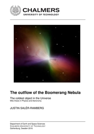
  • 1. The outflow of the Boomerang Nebula The coldest object in the Universe MSc thesis in Physics and Astronomy JUSTIN SALÉR-RAMBERG Department of Earth and Space Sciences CHALMERS UNIVERSITY OF TECHNOLOGY Gothenburg, Sweden 2016
  • 2.
  • 3. Master’s thesis 2016:NN The outflow of the Boomerang Nebula The coldest object in the Universe JUSTIN SALÉR-RAMBERG Department of Earth and Space Science Radio Astronomy and Astrophysics Chalmers University of Technology Gothenburg, Sweden 2016
  • 4. The outflow of the Boomerang Nebula The coldest object in the Universe JUSTIN SALÉR-RAMBERG © JUSTIN SALÉR-RAMBERG, 2016. Supervisors: Wouter Vlemmings and Theo Khouri, Department of Earth and Space Sciences Examiner: Wouter Vlemmings, Department of Earth and Space Sciences Master’s Thesis 2016:NN Department of Earth and Space Sciences Radio Astronomy and Astrophysics Chalmers University of Technology SE-412 96 Gothenburg Telephone +46 31 772 1000 Cover: An image of the Boomerang Nebula taken by the Hubble Space Telescope Typeset in LATEX Printed by [Name of printing company] Gothenburg, Sweden 2016 iv
  • 5. The Outflow of the Boomerang Nebula The coldest object in the Universe JUSTIN SALÉR-RAMBERG Department of Earth and Space Sciences Chalmers University of Technology Abstract The Boomerang Nebula is a preplanetary nebula with a massive and fast outflow. The gas in the outflow is seen as absorption against the cosmic microwave back- ground, making it the coldest known naturally occurring object in the Universe. Like an interstellar refrigerator, the outflow cools itself adiabatically. Old obser- vations with Swedish-ESO Submillimetre Telescope (SEST) were consistent with a constant-velocity outflow, but more recent observations, with Atacama Large Mil- limeter/submillimeter Array (ALMA), pointed to a model with an outflow velocity which varies radially. This thesis aims to reproduce the ALMA observations by considering two different scenarios, a scenario with an explosive event in which the material was ejected with a range of velocities and a scenario with an outflow with a time variable expansion velocity. The best-fit models for both scenarios produce similar spectra on the large scale, as the Boomerang Nebula in a larger region, but have difficulties matching the spectra along the line of sight through the center of the shell. The models that fit the data the best are similar too each other. The thesis also shows a model with a larger shell size than observed, that provides a good fit to the observations. While it is outside the scope of this thesis, it serves as a clue for future analysis of the Boomerang Nebula. Keywords: Stellar Physics, Astronomy, Stellar Winds, Outflow, Preplanetary Neb- ula v
  • 6.
  • 7. Acknowledgements First of all, I want to thank my supervisors Wouter Vlemmings and Theo Khouri who have dedicated a lot of time and effort to guide me along my thesis. They have had to answer to a lot of stupid questions and listen to a lot of stupid ideas. I want to thank them for not giving up and kept supporting me until the very end. Without their unwavering support this thesis would not have been possible. I want to thank the rest of the Star Formation and Evolved Star group for welcoming me into their circle and teaching me a lot about the field. I want to thank Ivan Marti-Vidal for a crash course in CASA python scripts. I want to thank the rest of the staff at Onsala Space Observatory for being among the most friendly, curious and dedicated people I have ever had the chance to meet. I am really grateful for the chance to spend half a year with you. I also want to thank my family for always supporting me. And most of all I want to thank my other half, Wenzhao Liu, for forcing me to work and helping me to relax. Justin Salér-Ramberg, Gothenburg, August 2016 vii
  • 8.
  • 9. Contents 1 Introduction 1 1.1 Units . . . . . . . . . . . . . . . . . . . . . . . . . . . . . . . . . . . . 2 1.2 Star formation and the main sequence . . . . . . . . . . . . . . . . . 3 1.3 Red giant branch and asymptotic giant branch . . . . . . . . . . . . . 5 1.4 Planetary nebulae . . . . . . . . . . . . . . . . . . . . . . . . . . . . . 5 1.5 Stellar effects on the ISM . . . . . . . . . . . . . . . . . . . . . . . . . 6 1.6 Boomerang Nebula . . . . . . . . . . . . . . . . . . . . . . . . . . . . 7 1.7 Probing the circumstellar environment . . . . . . . . . . . . . . . . . 8 1.8 Telescopes . . . . . . . . . . . . . . . . . . . . . . . . . . . . . . . . . 10 2 Stellar Winds 11 2.1 Heating and cooling processes . . . . . . . . . . . . . . . . . . . . . . 12 2.2 Photodissociation . . . . . . . . . . . . . . . . . . . . . . . . . . . . . 13 3 Motivation and methods 15 3.1 Outflow simulations . . . . . . . . . . . . . . . . . . . . . . . . . . . . 18 3.1.1 Explosion scenario . . . . . . . . . . . . . . . . . . . . . . . . 18 3.1.2 Decreasing velocity scenario . . . . . . . . . . . . . . . . . . . 19 3.1.3 Temperature profile . . . . . . . . . . . . . . . . . . . . . . . . 19 3.2 Radiative transfer . . . . . . . . . . . . . . . . . . . . . . . . . . . . . 19 4 Results 23 4.1 Explosion scenario . . . . . . . . . . . . . . . . . . . . . . . . . . . . 24 4.2 Decreasing velocity scenario . . . . . . . . . . . . . . . . . . . . . . . 31 4.3 Considering a large shell size . . . . . . . . . . . . . . . . . . . . . . . 34 5 Conclusion 39 5.1 Interpretation of Results . . . . . . . . . . . . . . . . . . . . . . . . . 39 5.2 Wind mechanism . . . . . . . . . . . . . . . . . . . . . . . . . . . . . 39 6 Future Prospects 43 Bibliography 45 ix
  • 11. List of Figures 1.1 A Hertzsprung Russel diagram showing the relationship between the luminosity and the temperature of a star. This plot clearly shows the main sequence full of young stars. The central star of the Boomerang Nebula is a post-AGB star. It has just left the AGB branch and is on it’s way to become a white dwarf. [1] . . . . . . . . . . . . . . . . 4 1.2 A schematic view of the AGB star during thermal pulses. Hydrogen burning happens in the envelope of the star producing helium. When enough helium has been created, helium burning is reignited pushing out the hydrogen envelope. . . . . . . . . . . . . . . . . . . . . . . . . 6 1.3 A schematic view of the Boomerang Nebula and its shell. The focus of this thesis is the Nebula’s absorbing outer shell, the coldest known naturally occurring object in the Universe. . . . . . . . . . . . . . . . 8 3.1 The spectra of the CO(J = 1 − 0) line from the SEST+ALMA data, given at four different apertures. The spectrum in the upper-left panel is similar to the SEST spectrum, while the spectrum in the lower-right panel was obtained from a much smaller aperture. . . . . 16 3.2 The first upper-left panel shows the CO(J = 1 − 0) line from a large aperture around the Boomerang Nebula. It is included to show how the original SEST data looked like. From the spectrum, it is hard to say anything about the velocity’s radial behavior. In the center of the line, there is emission from the inner shell. The upper-right panel shows the same line for a constant velocity model, to show that it is possible to describe the SEST data with it. The lower-left panel shows the CO line extracted from the ALMA data using an aperture smaller than the shell. The lower-right panel shows how a constant velocity model would look in the same aperture. A constant velocity model is not able to describe the ALMA spectrum and, hence, a model with a radially dependent velocity profile is required. . . . . . . . . . . . . . 17 3.3 How the simulation determined if two mass bins collided. The parti- cles had positions ri and rj and velocities υi and υj respectively. . . . 18 4.1 The logarithm of the density for an explosion model. The explosion used the parameters υc = 120km/s and υo = 100 km/s (see Equation (3.3)). The total gas mass is M = 2.9M . The model includes an AGB wind moving at a velocity of 15 km/s and has a mass loss rate of ˙M ≈ 10−5 M /year. . . . . . . . . . . . . . . . . . . . . . . . . . . 24 xi
  • 12. List of Figures 4.2 The temperature profile for an explosive wind colliding with an AGB wind. Th explosion uses the parameters υc = 120km/s and υo = 100 km/s (see Equation (3.3)) and the total gas mass is 1.4M . The AGB wind has a velocity at 15 km/s and a mass loss rate rate of ˙M ≈ 10−5 M /year. . . . . . . . . . . . . . . . . . . . . . . . . . . . . 25 4.3 Spectra for an explosion scenario model with an AGB wind, at differ- ent times. The explosion model has parameters υc = 120 km/s and υo = 100 km/s (see Equation (3.3)) and a total mass of 2.9 M . The AGB wind is moving at a constant velocity of 15 km/s and had a mass loss rate of 10−5 M /year. After 1150 years, the AGB wind has left the shell. . . . . . . . . . . . . . . . . . . . . . . . . . . . . . . . 25 4.4 The Gaussian distribution of an explosion with υc = 120 km/s and υo = 40 km/s. The velocity at the outer edge of the cold shell is υout = υc +2υo and the velocity at it’s inner edge is υin. At this time, most of the mass from the explosion is inside the shell. . . . . . . . . 26 4.5 The density profile for different parameters in the explosion scenario. The time is chosen accordingly to Equation (4.1). The profiles are compared to ρ ∝ r−2 , the density profile for a constant wind velocity. 27 4.6 The temperature profile for different velocity parameters, υo and υc, in the explosion model. The time is chosen accordingly to Equation (4.1). The temperature asymptotes T ∝ r−4/3 , the case of constant velocity without molecular heating, as the outflow velocity increases and the photoelectric heating weakens. . . . . . . . . . . . . . . . . . 27 4.7 The absolute value of the different heating and cooling mechanisms in the explosion scenario, 1040 years after the initial explosion. The parameters υc = 100 km/s and υo = 60 km/s, see Equation (3.3).The total gas mass in the explosion is 1.4M . . . . . . . . . . . . . . . . . 28 4.8 The intensity map of an outflow with the explosion scenario, 1150 years after the initial explosion. The parameters υc = 220 km/s and υo = 120km/s, see Equation (3.3).The total gas mass in the explosion is 2.9M . The color map is for velocities at υ = 0.5 km/s . . . . . . 28 4.9 Spectra from the explosion scenario, for different values of υc. The total gas mass is M = 2.9M . The offset velocity is υo = 100 km/s. . 29 4.10 Spectra from the explosion scenario for different values of υc. The total gas mass is M = 2.9M . The offset velocity is υo = 40 km/s. . . 29 4.11 Spectra from the explosion scenario for different values of υo. The total gas mass is M = 2.9M . The central velocity is υc = 120 km/s. 30 4.12 Spectra from the explosion scenario for different gas mass M. The central velocity is υc = 120 km/s and the offset velocity is υo = 100 km/s. . . . . . . . . . . . . . . . . . . . . . . . . . . . . . . . . . . . 30 4.13 The best fit of the explosion scenario to the SEST+ALMA data. This model has υc = 120 km/s, υo = 100 km/s and M = 1.8M . . . . . . . 30 4.14 The radial velocity profile for different ejection velocity parameters, vi and α. As α increases, the velocity profile becomes linear. . . . . . 32 4.15 The radial density profile for different ejection velocity parameters, vi and α. The density is much steeper than a constant velocity model. 32 xii
  • 13. List of Figures 4.16 The radial temperature profile for different ejection velocity param- eters, vi and α. The temperature approaches T ∝ r−4/3 , when υi increases, which is the case of a constant velocity and no heating. . . 33 4.17 The absolute value of the heating and cooling mechanisms in the decreasing model, with t = 1388 years and υ(r = 0, t) = 165 ∗ t−0.5 km/s. The dominant heating factor is the photoelectric heating, just weaker than the adiabatic cooling. . . . . . . . . . . . . . . . . . . . . 33 4.18 The spectra of υ(r = 0, t) = 165(t/year)−α km/s, where α is varied between 0.1 and 1. The spectra are taken when the front of the gas reaches the outer edge of the outer shell. . . . . . . . . . . . . . . . . 34 4.19 The spectra of υ(r = 0) = υi(t/year)−0.8 , where υi is varied. The spectra are taken when the front of the gas reaches the outer edge of the outer shell. . . . . . . . . . . . . . . . . . . . . . . . . . . . . . . 35 4.20 The spectra of υ(r = 0) = 200(t/year)−0.8 km/s, where the shell mass is varied. The spectra are taken when the front of the gas reaches the outer edge of the outer shell. . . . . . . . . . . . . . . . . . . . . . . . 35 4.21 The best fit for the decreasing wind scenario to the SEST+ALMA data. The ejection velocity is υ(r = 0) = 200(t/year)−0.8 km/s and a shell mass 2.97M . . . . . . . . . . . . . . . . . . . . . . . . . . . . . 36 4.22 The fit of an explosion model where the outer shell has a radius 75 . The velocity parameters are vc = 160 km/s and vo = 60 km/s. The total gas mass in the ejection is 2.9M . . . . . . . . . . . . . . . . . . 37 5.1 The spectra from the two scenarios’ best models. The explosion model was ejected instantly with a Gaussian velocity distribution with the central velocity, vc = 100 km/s and the velocity offset, vo = 60 km/s. The total mass in the explosion was 1.4M . The time decrease model used an ejection velocity v(r = 0, t) = 200(t/year)( − 0.8) and a shell mass 2.97M . . . . . . . . . . . . . . . . . . . . . . . . . . . . . . . . 40 5.2 The velocity, density and temperature profiles from the two scenarios’ best models. The explosion model was ejected instantly with a Gaus- sian velocity distribution with the central velocity, vc = 100 km/s and the velocity offset, vo = 60 km/s. The total mass in the explo- sion was 1.4M . The time decrease model used an ejection velocity v(r = 0, t) = 200(t/year)( − 0.8) and a shell mass 2.97M . . . . . . . 40 xiii
  • 15. 1 Introduction Stars are massive interstellar nuclear reactors in which new elements are created [1]. Without the stars there would not be any heavy elements. " We are all made of stardust " is an often repeated quote. Without the processes that occur in the stars, the giant element factories in the sky, there would be no Earth and there would not be any humans. The stars have an important role in the Universe and for life. That makes it very important to study them. More than 400 years have passed since Giordano Bruno realized that the stars and the Sun were the same type of entity [1]. He was the first to propose that stars, just like the Sun, have their own planets and other objects orbiting them. There was an easy way to learn more about stars right in our back alley, by investigating our own star, the Sun. In the last 400 years our understanding has increased vastly and recently more advanced telescopes and computers have made it easier for astronomers to study the stars. Nonetheless, there are still gaps to be filled by avid researchers. A lot is known about Sun-like stars, but exotic objects are often poorly understood. With more accurate telescopes distinct behaviors can be revealed, hidden in previous observations. Stars, just like living beings, evolve through several phases [1]. A star spends most of its lifetime on what is called the main sequence, in hydrostatic equilibrium. Hy- drostatic equilibrium implies that the nuclear fusion inside the star counterbalances the gravitational forces, preventing the star from imploding. When the nuclear fuel has been depleted within the core, the stellar structure readjusts to maintain the equilibrium. Stars with masses close to our Sun grows into giant stars with high mass loss rates [2]. After the star has ejected most of its material, the remnants of the central star can ionize it. With old telescopes, the ionized envelope looked similar to giant gas planets and is earning them the name "planetary nebula". The target of this thesis is the Boomerang Nebula which is a preplanetary nebula. In Preplanetary nebulae the outflow has not yet been ionized [3]. Compared to other preplanetary nebulae, the Boomerang Nebula holds several distinguishing features that separate it from its kin. Its rarest feature is its outflow which is the coldest known naturally occurring medium in the Universe [4]. The Boomerang Nebula was first observed in detail by Sahai and Nyman 1995 [4]. To fit the observations, they constructed a model with an assumption that the outflow had a constant velocity in the cold region. However new measurements from 2013 showed a multitude of velocities [5]. The velocity of the outflow had to have a radial dependence. The main goal of this thesis is to obtain a deeper understanding of the radial dependence of the outflow velocity. By understanding the behavior of unique 1
  • 16. 1. Introduction objects such as the Boomerang Nebula, we will improve our understanding of the late phases of stellar evolution. The first chapter is an introduction chapter, which gives a quantitative description and introduces the reader to the subject. It covers the units that are used in as- tronomy, as well as a short tour of stellar evolution. The third chapter’s focus is stellar wind models and how they can be used to describe the Boomerang Nebula’s outflow. The fourth chapter contains the motivation to this thesis and a description of the methods. The fifth chapter shows the result of the modelling and comparisons with observations. In the sixth chapter the results are discussed. The seventh and final chapter gives an outlook on future uses of the work in this thesis. It also covers potential upgrades to the models and the next steps necessary to understand the Boomerang Nebula. 1.1 Units It is no longer convenient to use standard SI units when working with the large scales in astronomy. While a meter or a kilogram works great when dealing with every day life, larger units are required when working with the large scales of the Universe. For example, astronomers count mass in solar masses, M [1]. A solar mass is M = 1.989 × 1030 kg. (1.1) The lifetime of a star is in scales of millions or billions of years, so during a second only an insignificant amount of mass is lost. The commonly used unit used for mass-loss rate of stars is M /year [1], where 1M /year = 6.305 × 10²² kg/s. (1.2) The movement of stellar objects tends to be estimated in kilometers per second. Giant stars can eject material moving at 500 km/s. Comparatively the speed of a bullet is 1 km/s. And while a bullet hits a wall within a few seconds, the ejected material moves freely. During a year, a short time compared to the stellar lifetimes, the ejected material travels 2 × 10¹⁰ km. During the same time starlight travels 9 × 10¹² km. These distances, which normally would seem immense, are quite small in the Universe. Measuring the large distances light and matter travel in space requires much larger units than measuring distances on Earth. Different units are chosen based on context. For describing the close environment of a stellar object, the common choice is astronomical units (AU), where 1 AU = 1.496 × 10¹¹ m. (1.3) 1 AU is the distance between the Earth and the Sun, or more explicitly since the Earth’s orbit around the Sun is elliptical, it is defined as the average of the minimum and maximum distance between them [1]. Initially this distance was calculated using the parallax method, which is still used to calculate the distance to stars. The parallax method uses the angle between a near object and a distant object [1]. When the observer moves, the nearer object seems to move with respect to the 2
  • 17. 1. Introduction farther away one. With the distant object as a reference point, the change in the angle between the two points can be noted. The parallax angle, p, is defined as half this change in angle, and with triangulation the distance to the nearby object is D = d tan(p) , (1.4) where d is half the distance between the observation points. The distance to other stars is so large that the parallax between two locations on earth is too small to be measured accurately. Instead the parallax angle is observed with a six month interval. In this time the Earth has travelled halfway around the Sun so that d = 1 AU. This distance is many magnitude larger than the Earth radius giving much more accurate results. But even when using the orbit of the earth, the parallax angle is still very small. Instead of degrees, astronomers use arc minutes and arc seconds for the parallax angle. An arc minute, or 1 , is defined as one sixtieth of a degree and similarly an arc second, or 1 , is one sixtieth arc minute. The unit for the distance to stars is 1 parsec = 1 AU tan(1 ) = 3.086 × 10¹⁶ m, (1.5) These units are necessary to know for reading astronomy papers, but more important to understand are the processes in the Galaxy. Next follows an introduction of the creation of the stars and their impact on the Galaxy. 1.2 Star formation and the main sequence Our galaxy is not only stars and empty space. The medium between the stars, called the interstellar medium (ISM), contains gas and dust [6]. 91% of the gas atoms in the ISM are hydrogen. The second most prevalent element in the ISM is helium, accounting for most of the remaining 9%. The relationship between stars and the gas is cyclical, the stars are born from the gas and during their lifetime the stars push it back into space. More specifically, stars are born within giant molecular clouds (GMCs). GMCs are humongous clouds of molecular gas, with diameters up too 100 parsec [7]. Just like stars, the GMCs are in hydrostatic equilibrium [6]. But eventually instabilities within the cloud lead to the collapse of pockets of gas. The molecular gas from the GMC is condensed in a few dense cores. At the center of each core a protostar forms. The accreted material have small rotational velocities which, to preserve the angular momentum, cause the cores to spin faster and faster. Like a pizza, the cores flatten and form a preplanetary disc around the protostar. The protostar starts ejecting matter perpendicular to its rotation. As the preplanetary disc spins, the dust in the disc combines into larger and larger grains of dust. After millions of years, most of the dust has bundled together into planets and other objects such as asteroids. In the protostar, the compression due to gravity leads to an increase in density, temperature and pressure. When the pressure is high enough to counterbalance 3
  • 18. 1. Introduction Figure 1.1: A Hertzsprung Russel diagram showing the relationship between the luminosity and the temperature of a star. This plot clearly shows the main sequence full of young stars. The central star of the Boomerang Nebula is a post-AGB star. It has just left the AGB branch and is on it’s way to become a white dwarf. [1] the gravity the cloud regains hydrostatic equilibrium. The collapse stops, but the protostar is too cold for nuclear fusion. At a temperature of around 2000 K , the thermal energy causes the molecular hydrogen inside the nucleus of the core to dissociate [8]. Soon after, the hydrogen and the helium are ionized, and at 107 K, the Star’s nucleosynthesis can start [9]. At the protostar’s nucleus the hydrogen atoms fuse into helium, releasing energy. Since this process is exothermic, it is called hydrogen burning. When the hydrogen burning starts the protostar has transformed into a star. The newborn star is located on the main sequence, where it will spend 90 % of its lifetime [1]. Stars in the main sequence are in hydrostatic and thermal equilibrium. Thermal equilibrium states that the energy generation of the star is balanced by it’s luminosity. The correlation between stars in the main sequence can be seen in a Hertzsprung-Russel (HR) diagram (see Figure 1.1). The HR diagram shows the relationship between the luminosity and the effective temperature of the stars. Depending on a star’s position on the HR diagram its evolutionary phase can be inferred. 4
  • 19. 1. Introduction When the nucleus of a main sequence star is depleted of hydrogen, it is impossible for hydrogen burning to continue within it [3]. With no hydrogen burning, there is no pressure to balance out the gravity. This causes the nucleus to lose hydrostatic equilibrium and collapse. The gravitational energy is converted into thermal energy, increasing the temperature and triggering hydrogen burning in a shell around the core. The helium produced in the shell falls back into the core, increasing the core’s density and temperature. 1.3 Red giant branch and asymptotic giant branch The higher temperature enables higher rates of hydrogen burning in the shell than earlier within the nucleus. The increase in energy output causes the star to expand to several magnitudes bigger than its main sequence size. As the surface area of the star increases the surface temperature decreases. The nucleus is hot and massive, while the star has a low effective temperature and a critically low density. Due to the color and the size of the star, it is labeled as a red giant. Red giants are located on the red giant branch (RGB) in the HR diagram (Figure 1.1). When the nucleus has reached a temperature of 108 K the helium fuses into beryllium [3]. Through fusing with other helium atoms, it forms carbon and then oxygen. Dur- ing this process, called helium burning, the star’s effective temperature is increasing with conserved luminosity. The star simultaneously burns helium in its nucleus and hydrogen in a shell. After this phase, called the horizontal branch (HB), the star enters the asymptotic giant branch (AGB). During the HB, the nucleus expends its helium [3]. Left in the nucleus is carbon and oxygen, with too low temperature for them to fuse. Instead helium burning starts in a shell around the nucleus. The star is again a red giant. The AGB is said to be asymptotic since it approaches the RGB asymptotically in the HR diagram. After the helium shell is depleted, the star derives its energy from hydrogen burn- ing in a thin hydrogen shell [2]. The helium produced forms a thin layer of helium between the hydrogen shell and the nucleus. When enough helium has been accumu- lated, helium burning is reignited. The helium burning will push out the hydrogen shell and extinguish the burning there. This process is referred to as a thermal pulse. After the thermal pulse, hydrogen burning is reignited in the the shell accumulating more helium for another thermal pulse (see Figure 1.2). Thermal pulses increase the luminosity and size of the star periodically. During the pulses, and to a lesser extent during the entire AGB phase, a lot of mass is ejected into the star’s circumstellar environment. 1.4 Planetary nebulae When an AGB star has ejected almost all of its hydrogen envelope, it will enter the preplanetary nebula (PPN) phase [2]. When looking at PPNs, the focus does not lie on the central star, but instead on the ejected material. This is because the ejected gas can be many times the mass of the star. 5
  • 20. 1. Introduction Figure 1.2: A schematic view of the AGB star during thermal pulses. Hydrogen burning happens in the envelope of the star producing helium. When enough helium has been created, helium burning is reignited pushing out the hydrogen envelope. During the PPN phase, the central star is too cold to ionize the ejected material. Preplanetary nebulae are said to be reflection nebulae. Reflection nebulae have very little emission in the visible spectra and were originally detected by the scattering of the light from their central stars. From the hydrogen burning in the shell, the star’s effective temperature is increasing. When the central star has become hot enough to produce ultraviolet light, it ionizes the ejected envelope. The ionized envelope becomes an emission nebula, showing an appearance similar to giant gas planets such as Jupiter. The star has entered the planetary nebula (PN) phase. The PN phase is the star’s last high-luminosity phase. When the hydrogen shell exhausts, the central star becomes too cold to ionize its increasingly distant gas cloud and become a white dwarf. White dwarfs are dense stars, with no internal source of energy. Meanwhile the gas cloud turns invisible, ending the planetary nebula phase. Planetary nebulae comes in various shapes [10]. Everything from bipolar and disc- shaped to quadripolar and point-symmetric planetary nebulae have been observed. The morphology of the planetary nebulae is highly dependent by how it acts during the PPN phase. One of the reasons to study the Boomerang Nebula is to understand how the shaping of PN takes place. 1.5 Stellar effects on the ISM While most stars enter the RGB after depleting hydrogen in their nuclei, not all of them do. Main sequence stars with a mass below 0.5 M never become hot enough to initiate helium burning. Instead they cool down and turn into white dwarfs [1]. Stars with high mass also have unique features, main sequence stars heavier than 6
  • 21. 1. Introduction 2 M smoothly proceeds with helium burning after the hydrogen is depleted. They then have helium burning and hydrogen burning in their shell simultaneously. Stars with a main sequence mass above 8M are able to burn the carbon within its core to produce magnesium [2]. Heavier elements are produced in supergiants , stars with main sequence masses above 10M , named as they grow much larger than other stars [11]. Super giants are composed of several shells, each with different elements burning, and eventually build up an iron nucleus [12]. When a super giant depletes its fuel, it collapses into a supernova. Supernovae are titanic explosions able to outshine entire galaxies [1]. The total radiant energy of a supernovae is the same as our Sun will produce during its entire life. The high energy of supernovae make them the most energetic nuclear reactors in the Universe. Most natural elements heavier than iron are produced in supernovae. The exception is specific elements created through slow neutron capture processes in AGB stars’ shell. From the chemical composition of the ISM it is possible to learn about nearby stars. While most helium and hydrogen were created in the Big Bang, heavier elements are often created in stars [1]. And generally, the heavier an element is, the bigger was the nuclear reactor it was produced in. It is not only gas that the stars eject into ISM, but also dust. Most of the cosmic dust in the ISM is formed in AGB stars or supernovae [2]. Just like the gas can be traced to its progenitors, so can the dust. Stars with more oxygen than carbon produce oxygen rich dust, oxides and silicates, and stars with more carbon produce carbon rich dust, carbocaneous dust. Supernovae have both carbon rich and oxygen rich layers and therefore can produce both kind of dust. But since most of the layers are oxygen rich, the dust from supernovae are dominantly silicates. All AGB stars are initially oxygen rich, But AGB stars with a mass between ≈ 1.6M to 4M will become carbon rich. Therefore, the surrounding dust contain information about the chemical structure of the stars, as well as limits to an AGB star’s mass. 1.6 Boomerang Nebula The Boomerang Nebula is a biconal preplanetary nebula, discovered by Wegner and Glass in 1979 [13]. Its most unique feature is its outflow, which is the coldest known natural occurring object in the entire Universe [4]. As a remnant of the Big Bang, the Universe is coated with Cosmic Microwave Background Radiation (CMBR), with a characteristic temperature around 2.7 K. Normally the CMBR has to be treated as noise, as the emission from stars towers about it, but the Boomerang Nebula’s outflow is cold enough to absorb the photons emitted from the CMBR. By absorbing the CMBR photons, the outflow is self-shielded and the CMBR photons can not penetrate and heat the innermost regions. Another interesting aspect of the Boomerang Nebula, and bipolar nebulae in general, is that the outflow seems to carry a much larger amount of linear momentum than expected from the current model for radiation-pressure-driven outflows in evolved stars. The mechanism behind the driving of these winds is not understood and is one of the reasons for studying these enigmatic objects [14]. 7
  • 22. 1. Introduction Figure 1.3: A schematic view of the Boomerang Nebula and its shell. The focus of this thesis is the Nebula’s absorbing outer shell, the coldest known naturally occurring object in the Universe. The outflow of the Boomerang Nebula is separated in two distinct shells [4], illus- trated in Figure 1.3. The inner shell is biconal, with a temperature slightly above the CMBR and a velocity around 35 km/s. It is located between 2.5 (3743 AU) and 6 (8690 AU) from the central star. The outer shell, which is colder than the CMBR, is located between 6 (8690 AU) and 33 (48129 AU). It does not follow the biconal shape of the inside and is instead almost spherical. The outer shell has a multitudes of velocities, peaking at around 165 km/s. In the outflow, the hydrogen has returned to its molecular state. Even if hydrogen is the most dominant element in the molecular gas, molecular hydrogen has no permanent dipole moment [6]. It radiates very poorly at radio wavelengths, making it difficult to detect. Due to this, other molecules are used to trace the outflow. A good tracer is carbon monoxide (CO). CO has stable bonds and several emissions in the radio spectrum. 1.7 Probing the circumstellar environment When a molecule changes state, it absorbs or emits a photon [15]. These photons, detectable with telescopes, give us information about distant objects. The energy levels, or states, of the molecules are quantized so that when a molecule absorbs or emits a photon, its frequency and energy can be related to a state transition. Molecules have three different kinds of state transitions [15]. The most energetic transitions are electronical. These transitions happen when the electrons inside the molecules are excited or deexcited, emitting UV photons. The second most energetic are the vibrational transitions. When the molecules transit between vi- brational states they emit infrared (IR) photons. The least energetic transitions of the molecules are the rotational transitions. The rotational transitions emit photons in the radio, sub-millimeter and IR wavelengths. Radio photons can be detected on 8
  • 23. 1. Introduction the Earth’s surface, while UV and IR photons are blocked by the atmosphere. Due to this, the rotational transitions are often the ones that can be observed in the greatest detail. Rotational transitions can be modelled as a rigid rotor [1]. In classical physics the energy of a rigid rotor is Erot = L2 2I , where L is the angular momentum and I is the rotor’s moment of inertia. Similarly the energy of the rotation states are E(J) = J(J + 1)h2 8π2I = B0J(J + 1). (1.6) In this equation, J is the quantum number for the rotational states, with J = 0 being the rotational ground state. Linear molecules, like CO, follows the rotational transition rule, ∆J ± 1. The constant, h, in the equation is Planck’s constant. The energy of a photon that is emitted from J → J − 1 is Ephoton = ∆E(J) = E(J) − E(J − 1) = B0(J(J + 1) − J(J − 1)) = 2B0J. (1.7) For example, CO has the rotational constant B0 = 0.238 meV [6]. Equation (1.7) then states that the rotational transition CO(J = 1 → 0) emits a photon with an energy of 0.476 meV. From Planck’s relation the frequency of the photon is 115.27 GHz. Planck’s relation correlates the energy, Ephoton with the frequency, ν as Ephoton = hν. (1.8) The emission lines can be used to obtain the target’s minimum temperature [6]. The thermal energy of an object is given as Et = kBT, where kB is the Boltzmann constant and T is the target’s temperature. For example, for CO to continually emit CO(J = 2 → 1), the molecules need to be excited to the second rotational level. Using Equation (1.6) and B0 = 0.238 meV, T ≥ 6B0 kb = 16.6 K. Normally the emission source is moving, so that the frequency will be shifted by the Doppler effect [1]. The Doppler effect is a relativistic effect. It states that if the emission source is moving at a velocity, ∆υ, relative to the observer, the observer sees a photon with frequency νc = ν0(1 + ∆υ c ). (1.9) Here, c, is the speed of light and, ν0, is the emission frequency excluding the Doppler effect. While it may require more than one emission peak to find ∆υ, the relative velocity is useful information of the target. The Doppler effect also has another impact on the emission line. Since the Doppler shift perceived by an observer is determined by the velocity component along the line of sight, different regions of a circumstellar envelope expanding with velocity υ will present different Doppler shifts. A given observed line is said to be broadened by this effect. The projected velocity changes gradually from −υ for gas in the part of the envelope moving away from the observer to 0 in the plane of the sky to υ in the part of the envelope approaching the observer. On top of this, any radial variations of the expansion velocity may also contribute to the broadening of a given line. 9
  • 24. 1. Introduction 1.8 Telescopes Measuring the emission lines of stellar objects, thousands of parsecs away, requires large telescopes with advanced equipments. The angular resolution of a telescope is inversely proportional to its aperture diameter [16]. This thesis uses data sets obtained with two different telescopes. The first was obtained in 1997 by Sahai and Nyman with the Swedish-ESO Submillimeter Tele- scope (SEST) [4]. SEST was a radio telescope in La Silla, Chile, that was active between 1987 and 2003 [17]. It had an aperture diameter of 15 m and, for the CO(J = 1 − 0), an angular resolution of 42 . As the Angular resolution was larger than the Boomerang Nebula (see Figure 1.3), the observation did not provide much details on the velocity dispersion. The second data set was obtained in 2013 by Sahai et al. with the Atacama Large Millimeter/submillimeter Array (ALMA) [5], also located in Chile. ALMA used an array of 33 telescopes to virtually increase the aperture. In total, ALMA has 55 telescopes [18], moveable to span an aperture with a diameter of 16 km. With ALMA, it was possible to reduce the angular resolution down to less than 5 , smaller than the outer shell. 10
  • 25. 2 Stellar Winds Outflows that originate from stellar atmospheres are called stellar winds [6]. The focus of this thesis is to model the velocity dependence of the outflow in the outer shell of the Boomerang Nebula. Stellar winds collide with gas in the ISM or the circumstellar envelope. These can usually be distinguished based on differences in parameters such as velocity, density and temperature. The goal of the wind model is to obtain such parameters for the Boomerang Nebula’s outflow. They can be obtained from radiative transfer model, since the emission from the outflow depends on its parameters. Stellar wind models assume that mass, momentum and energy are conserved [19]. The mass conservation can be modeled by the mass continuity equation ∂ρ(r) ∂t + · ρ(r)v(r) = 0. (2.1) The mass continuity equation has a spatial dependence, using r as the position vector. At r the density is ρ(r) and the outflow velocity is v(r). The mass continuity equation can be related to the star’s mass loss ˙M with two assumptions. The first assumption is spherical symmetry, that the outflow is sym- metric in all directions from the star. The distance to the center of the star r can replace r. The second assumption is that the system is in steady state. This means that the stellar wind properties are constant in time. Under these assumptions Equation (2.1) can be rewritten as ˙M = 4πρvr2 . (2.2) Equation (2.2) is irrelevant for an outflow with a radial dependence, but is useful for showing relations between parameters in stellar wind models. The second quantity that is conserved is momentum, for which the conservation equation is ∂v(r) ∂t + v(r) · v(r) = − P(r) ρ(r) − GM r2 ˆr. (2.3) P is the radiation pressure, G is Newton’s gravitational constant and M is the mass of the star. In the outer shell of the Boomerang Nebula we have a large distance and a high velocity. Due to this, the contributions from the pressure and gravity are negligible. Under these assumptions Equation (2.3) can be reduced to ∂v(r) ∂t + v(r) · v(r) = 0. (2.4) 11
  • 26. 2. Stellar Winds This equation can be fulfilled with simple Newtonian mechanics. It is assumed that the wind can move freely in space without outer constraints. It is simple to obtain the the radial dependencies of the density and velocity. But to obtain the radial profiles of the temperature, it is required to consider the heating and cooling processes in the outflow. 2.1 Heating and cooling processes The radial dependence of the temperature can be modeled as [20] dT(r) dr = (2 − 2γ)(1 + r 2v(r) ∂v(r) ∂r ) T(r) r + γ − 1 nH2 (r)kBv(r) (H − C). (2.5) The first term covers the adiabatic cooling. The adiabatic cooling is the dominant cooling process in the outflow, caused by pressure decrease in a system [21]. The common gas law states that a decrease in pressure makes it expand. But a system with neither matter or heat output is adiabatically isolated. When an adiabatically isolated system expands, it does work on its surrounding, cooling itself. In the adiabatic cooling term, T is the outflow temperature and γ is the heat capacity ratio. The heat capacity ratio can be related to the degrees of freedom of the gas, f, γ = f f + 2 . (2.6) At T ≤ 300, the rotational excitations of H2, the dominant molecules in the molec- ular gas, are insignificant. Due to this the molecular gas can be treated as a mono- atomic gas with f = 3 and γ = 5/3. The second term in Equation (2.5) contains the molecular heating and cooling pro- cesses in the outflow. Here nH2 is the number density of the molecular gas, which is related to the mass density by ρH2 = mH2 nH2 , where mH2 is the mass of a H2 molecule. The constant kB is the Boltzmann constant, relating the system’s thermal energy and temperature, Et = kBT. Finally H − C is the sum of the heating and cooling rates. The dominant heating processes are dust-gas collisional heating, dust-gas adhesion heating and photoelectric heating [22]. The dust-gas collisional heating [20] comes from gas colliding with dust and is mod- elled with Hdg = 3 8 mH2 (nH2 (r))2 Ψ agρg v3 drift 1 + vdrift v(r) . (2.7) The dust properties is the dust-to-gas mass ratio, Ψ, the average dust grain radius, ag and the average dust grain density, ρg. The model assumed silicate dust with Ψ = 0.01, ag = 0.1 µm and ρg = 3.3 g/cm3 . Another dust property is the drift velocity of the dust through the gas, vdrift. This is assumed to be constant at vdrift = 10 km/s. The dust adhesion heating [23] can be modelled as Hdt = 2.008×10⁻³¹ (nH2 (r))2 Ψ agρg T(r)(Tdust − T(r)(0.35e − Tdust+T (r) 500 +0.1). (2.8) 12
  • 27. 2. Stellar Winds The expression contains the dust temperature Tdust, which has been assumed to be constant at 15K. Note that the equation assumes SI units. The final heating contribution that was considered is the photo-electric heating, which is the heating of the gas from stray photons. It is covered in Hpe = KpenH2 (r), (2.9) where Kpe = 10−33 J/s [24]. The only non-adiabatic cooling term able to affect the temperature is the H2 vibra- tional line cooling [23], CH2 = 2.611 × 10⁻³⁴ nH2 (r)( Tkin 1000 )4.74 . (2.10) From putting all the heating and cooling factors together in Equation (2.5), the temperature’s radial dependence can be obtained. The photoelectric heating came from photons stimulating electronial transitions in the gas, but if the photons are energetic enough they are able to dissociate the molecular gas into atoms. 2.2 Photodissociation At the inner regions of the circumstellar envelope the molecules are shielded by the gas in the outer region. But in outer regions, the molecular bonds break from interactions with high energy photons from the ISM. At the so called dissociation radius, half of the molecules in the gas have dissociated. The dissociation radius varies between different molecules, relative to their dissociation energy, which is the minimum energy for a photon to dissociate it [25]. The high dissociation energy of CO is one of the properties that makes it a good tracer molecule. But even if the dissociation radius of CO is large, it is not infinite. Outside of its dissociation radius the CO dissociates into C and O atoms. And although the stellar wind continues, the CO emission or absorption lines dissappear. 13
  • 29. 3 Motivation and methods The Boomerang Nebula was initially discovered in 1978 by Wegner and Glass [13]. In 1997 its molecular outflow was observed by Sahai and Nyman with SEST (Swedish ESO Submillimeter Telescope) [4]. They discovered that the nebula’s outflow is colder than the cosmic microwave background radiation (CMBR). The CMBR is a remnant from the Big Bang maintaining the Universe’s temperature at 2.7 K. The outer shell of the Boomerang Nebula (see Figure 1.3) by mimicking the behavior of a refrigerator. It cools through adiabatic cooling and self-shields from the CMBR. But the Boomerang Nebula is not only colder than the CMBR, it is also the coldest known naturally occurring object. The SEST spectrum of the CO(J = 1 − 0) transition shows absorption in velocities ranging from roughly −165 km/s to 165 km/s. As explained at the end of Section 1.7, this is caused by Doppler line broadening and reflects the velocity dispersion in the shell. The SEST spectrum had a beam size of 40 , and resembled the first plot in Figure 3.1. It shows a wide velocity dispersion that could be explained using many different models. The emission at the center of the spectrum originates in the inner shell (see Figure 1.3) and is not considered in the thesis. Further observations of the Boomerang Nebula were done by Sahai et al. in 2013 with ALMA [5], which used an array of several telescopes to simulate a smaller beam size. The beam, which was not circular, had a major axis of 4.12 and it’s minor axis of 1.83 . Figure 3.1 depicts ALMA observations which show that even for smaller beam sizes, the outer shell shows absorption in a wide range of velocities. Sahai and Nyman constructed a model with a constant expansion velocity, that could fit well to the SEST spectrum (see figure 3.2) [4]. However, a constant velocity model produces two sharp absorption peaks when imaged with a small aperture (see the last plot in Figure 3.2), in contrast to what is seen in the ALMA observations. To address this problem, two different scenarios with radially dependent outflow velocities were considered. The first one is an initial explosion ejecting most of the gas into the envelope. The second scenario is an outflow with a time-varying ejection velocity. The scenarios were modelled independently and their parameters were adjusted to match the ALMA and SEST data. The outflow was simulated in MATLAB. Assuming spherical symmetry the outflow could be modelled with one dimensional mass bins. And assuming that the radia- tion pressure and gravitation had negligible effect, the gas could move freely. The outflow simulations output the radial profiles of velocity, density and temperature. The profiles were input into a radiative transfer (RT) model to simulate how light propagated inside the outflow. The RT model produced the CO(J = 1−0) line that 15
  • 30. 3. Motivation and methods Figure 3.1: The spectra of the CO(J = 1 − 0) line from the SEST+ALMA data, given at four different apertures. The spectrum in the upper-left panel is similar to the SEST spectrum, while the spectrum in the lower-right panel was obtained from a much smaller aperture. 16
  • 31. 3. Motivation and methods Figure 3.2: The first upper-left panel shows the CO(J = 1 − 0) line from a large aperture around the Boomerang Nebula. It is included to show how the original SEST data looked like. From the spectrum, it is hard to say anything about the velocity’s radial behavior. In the center of the line, there is emission from the inner shell. The upper-right panel shows the same line for a constant velocity model, to show that it is possible to describe the SEST data with it. The lower-left panel shows the CO line extracted from the ALMA data using an aperture smaller than the shell. The lower-right panel shows how a constant velocity model would look in the same aperture. A constant velocity model is not able to describe the ALMA spectrum and, hence, a model with a radially dependent velocity profile is required. 17
  • 32. 3. Motivation and methods Figure 3.3: How the simulation determined if two mass bins collided. The particles had positions ri and rj and velocities υi and υj respectively. were compared with the observations. 3.1 Outflow simulations The mass bins were ejected from the central star with an initial velocity that de- pended on the scenario. After a time step ∆t, a given mass bin located at ri with velocity υi moved to a new position. ri = ri + υ∆t. (3.1) The simulations included collisions when one mass bin encountered others. Given a second mass bin located at rj with velocity υj, it will collide with the first mass bin if rj ≤ ri and rj + vj∆t ≥ ri + vi∆t (see Figure 3.3). If these criteria were obeyed for several mass bins, it was treated as a multibody collision. In the simulations all mass bins had the same mass m and the collisions were considered elastic. Therefore after a collision, the mass bins had a velocity equal to their mean velocity. The velocity profile, υ(r), was the mean velocity of all mass bins between r and r + δr, where δr is the radial resolution. Similarly the density profile was ρ(r) = m 3dN 4π((r + δr)3 − r3) , (3.2) where dN is the amount of mass bins between r and r + δr and m is the mass of a mass bin. 3.1.1 Explosion scenario In the explosion scenario, all the mass bins were ejected at t = 0, with a Gaussian velocity distribution 18
  • 33. 3. Motivation and methods f(υ) = 1 υo √ 2π e −(υ−υc)2 2υ2 o . (3.3) Here υc is the central velocity and υo is the standard deviation of the distribution. The standard deviation is the square root of the expected value of (υ − υc)2 . These two parameters could be adjusted for matching the ALMA data. The third param- eter was the total ejected mass M, which was related to the density as M = mnbins. Here nbins is the total amount of mass bins in the model, and serves as a resolution parameter for the model. 3.1.2 Decreasing velocity scenario The second scenario used υ(r = 0) = υi( t t0 )−α , (3.4) where α and υi are adjustable parameters. The outflow starts ejecting at the time t0 with the initial ejection velocity υi. If α < 0 a snowplow effect would be created, gathering the gas in a single wavefront. This is inconsistent with the ALMA data, so α must be positive. It was also assumed that the mass loss rate ˙M was constant. The mass bin mass could be related to the mass loss rate as m = ˙Mdt, (3.5) where dt is the time difference between the ejection of two mass bins. Just like nbins, dt is another resolution parameter. The parameter used for scaling the density was Mshell, which is the mass that has entered the shell. Mshell = ˙M(dtshell), (3.6) where dtshell is the time between the ejection of the first and the last mass bins in the shell. 3.1.3 Temperature profile The temperature profile was calculated in the same way for both models, and re- quired the density and velocity profiles as input. At the inner edge of the cold region (see Figure 1.3), the temperature was set to the CMBR temperature, T(8690AU) = 2.725 K. Thereafter the temperature was integrated stepwise with the different heating contributions in Equation (2.5), T(r + dr) = T(r) + dT dr (r)dr. (3.7) 3.2 Radiative transfer The velocity, density and temperature profiles were input into a radiative transfer (RT) software called LIME [26]. RT is the study of how photons propagate within 19
  • 34. 3. Motivation and methods a medium. RT modelling can be done analytically for simple morphologies, but for more complex ones even numerical solutions require extensive calculations. LIME is a software created by C. Brinch and M. R. Hogerheijde for RT solutions at millimeter and far-infrared wavelengths [26]. LIME received as input the velocity, density and temperature profiles together with CO properties to create an image cube of the CO(J = 1 − 0) line. Image cubes contain the intensity as a function of longitude, latitude and the velocity along the line of sight. Spectra were extracted from the image cube with the Common Astron- omy Software Applications (CASA), an applications package constructed for data post-processing. The spectra were extracted from apertures with two different radii to examine the stellar wind parameters’ impact on the line shape. The parameters were then adjusted in an attempt to fit the ALMA data. LIME like other RT models is based on the equation of RT [1], dIν ds = jν − ανIν. (3.8) The equation of RT depicts how the intensity, Iν, in a given frequency, ν, changes along a path, s, through a medium. The parameters, jν and αν, are the emission coefficient and the absorption coefficient, based on the medium along the path [1]. The coefficients differ for dust and for gas, where the dust-to-gas ratio was assumed to be 0.01. For gas jgas ν = hν 4π n2A12Φ(ν) αgas ν = hν 4π (n1B12 − n2B21)Φ(ν), (3.9) where A12, B12 and B21 are the Einstein coefficients [26], which define the emission and absorption probabilities for a transition between two states with densities, n1 and n2. A12 is the probability of spontaneous emission, B12 of absorption and B21 of stimulated emission. The energy difference between the states is E2 − E1 = ∆E = hν, with h as Planck’s constant. The function Φ(ν) is a line broadening function built on several mechanisms, with the dominant mechanism being the Doppler line broadening from the velocity dispersion. The emission and absorption coefficients in dust are jdust ν = −αgas ν Bν(Tdust) αdust ν = κνρdust. (3.10) For calculating the dust coefficients, the dust opacity, κν, the dust temperature, Tdust, and the dust density, ρdust, are necessary. The dust opacity were input into the model, Tdust was assumed as equal to the gas temperature, Tgas, and ρdust was related to the gas density by the dust-to-gas ratio. The dust parameters were chosen with the assumption of that the dust was silicate dust. Bν is the black body function. The local mean radiation field was retrieved from integrating the intensity over all solid angles, Jν = (4π)−1 IνdΩ. (3.11) 20
  • 35. 3. Motivation and methods The mean radiation field was used together with the collisional excitation or de- excitation rate Cil, between two states, i and l, to calculate the state population [26] ni = l>i nlAli + l=i nl(BliJli + Cli) l<i Ail + l=i(BilJil + Cil) , Cil = gl gi cile −hc kBTgas (El−Ei) . (3.12) The statistical weights, gl and gi, and the rate coefficients, cil, are input param- eters in the model when calculating, Cil. The constants in the equations are the Boltzmann constant, kB, and the light speed in vacuum, c. The Equations (3.8), (3.9), (3.11) and (3.12) create a recursive problems serving as a baseline for the LIME code. The LIME code also accounts for Doppler shifts between different regions of the envelope. 21
  • 36. 3. Motivation and methods 22
  • 37. 4 Results Two scenarios were modelled. An explosion scenario, where all the matter is ejected simultaneously and a scenario with an outflow with an ejection velocity that de- creased with time. While the outflow in both scenarios started close to the central star, the profiles were modelled in the outer shell. The outer shell is the cold region in the Boomerang Nebula ranging from rin = 8.7 × 10³ AU (6 ) to rout = 48 × 103 AU (33 ), see Figure 1.3. From the stellar wind models radial profiles of velocity, density and temperature were calculated. These were input into a radiative transfer (RT) model to create image cubes. CASA, the Common Astronomy Software Applications package, was used to extract the CO(J = 1−0) line shapes from the image cubes. The line shapes were calculated from two circular apertures, with radii r1 = 3 and r2 = 30 . These apertures can be compared to the ALMA data and the SEST data, respectively. The smaller aperture provides the line of sight absorption, where the larger aperture grants us the total velocity dispersion in the Nebula. Initially, the models included an earlier slow AGB wind to be swept up by the ejection. The slow wind was given a velocity of 15 km/s and a mass loss rate rate 10−5 M /year, based on typical parameters for the outflow from AGB stars. Figure 4.1 shows how the density would behave with the presence of an AGB wind in the explosion scenario. When the fast ejecta collides with the AGB wind, the velocity at the wind front decreases. As the AGB wind gets swept up, a density peak is formed at the wind front (see Figure 4.1). The observation does not show any signs of shock features. Another argument for there being no traces of the previous AGB wind inside the cold shell is that it is too slow to cool adiabatically. An AGB wind would have a temperature higher than the CMBR (see Figure 4.2). At low velocities the adiabatic cooling is too weak to counterbalance the photoelectric effect, so such an AGB wind can not absorb against the CMBR. Figure 4.3 shows spectra at different times with an explosive wind colliding with an AGB wind. Before 1150 years, the constant AGB wind is still present in the shell, appearing as a thin line at low velocities. This feature is missing from the observations. Hence ,the AGB wind needs to have a very low mass loss rate, leading to a very small effect on the fast ejecta. Another possible scenario is that the previous AGB wind already has left the shell and have dissociated or heated up to the background temperature. As Figure 4.3 shows the spectra depends on the life time of the Nebula, but it was not treated as a free parameter. The gas at rout may still be colder than the CMBR, so it was assumed that the fast-velocity ejected gas just filled the shell. In the velocity decrease scenario, this happens when the fastest mass bin reaches rout. For 23
  • 38. 4. Results Figure 4.1: The logarithm of the density for an explosion model. The explosion used the parameters υc = 120 km/s and υo = 100 km/s (see Equation (3.3)). The total gas mass is M = 2.9M . The model includes an AGB wind moving at a velocity of 15 km/s and has a mass loss rate of ˙M ≈ 10−5 M /year. the explosion scenario, however, this time is not always straight-forward to define, see discussion below. 4.1 Explosion scenario Technically the shell is full when the fastest mass bin reaches rout. But in the case of a Gaussian velocity distribution, the maximum velocity depends on the amount of the mass bins. Hypothetically, if our simulation used an infinite amount of mass bins, the maximum velocity would also be infinite. But the fraction of mass bins at high velocities are very low, see Figure 4.4, so the density at the edge of the shell would be too low to significantly affect the line shape. Instead, what was chosen was t = rout/(υc + 2υo). (4.1) At this time only ≈ 2.5% of the total mass has passed rout. Meanwhile, as seen in 4.4, a significant fraction of the mass bins has passed rin, so that most of the mass from the explosion has reached the outer shell. On the one hand, the velocity profile was independent of the parameters of the initial velocity distribution, since an instant ejection generates a linear velocity profile v = r/t. (4.2) On the other hand, the density profile depends significantly on the parameters of the initial velocity distribution. Figure 4.5 shows how the density profile changes with 24
  • 39. 4. Results Figure 4.2: The temperature profile for an explosive wind colliding with an AGB wind. Th explosion uses the parameters υc = 120km/s and υo = 100 km/s (see Equation (3.3)) and the total gas mass is 1.4M . The AGB wind has a velocity at 15 km/s and a mass loss rate rate of ˙M ≈ 10−5 M /year. Figure 4.3: Spectra for an explosion scenario model with an AGB wind, at different times. The explosion model has parameters υc = 120 km/s and υo = 100 km/s (see Equation (3.3)) and a total mass of 2.9M . The AGB wind is moving at a constant velocity of 15 km/s and had a mass loss rate of 10−5 M /year. After 1150 years, the AGB wind has left the shell. 25
  • 40. 4. Results Figure 4.4: The Gaussian distribution of an explosion with υc = 120 km/s and υo = 40 km/s. The velocity at the outer edge of the cold shell is υout = υc + 2υo and the velocity at it’s inner edge is υin. At this time, most of the mass from the explosion is inside the shell. the velocity parameters and the total gas mass M. The smaller υo in comparison to υc, the more apparent is the effect of the initial velocity distribution. It appears as a bulge compared to the constant velocity density, ρ ∝ r−2 .But when υo is large compared to υc, υc has little effect on the density. The total gas mass, M, only serves as a scaling parameter for the density. As seen in figure 4.7, the dominant heating effect in the outflow is the photoelec- tric heating. Equations (2.5) and (2.9) states how its effect on the temperature is inversely proportional to v. Since the main component of the adiabatic cooling (see Equation (2.5)) only depends on r, Figure 4.6 shows how the temperature ap- proaches T ∝ r−4/3 , the case with only adiabatic cooling, as the outflow velocity, υc or υo, increases. The temperature varies very little with the gas mass M, since the density dependent heating factors in Figure 4.7 have little impact on the outflow temperature. The radiative transfer (RT) software created intensity image cubes from the radial profiles, containing absorption intensity for different observations angles and veloci- ties. The spatial dependence of the absorption from an explosion model can be seen in Figure 4.8. The Doppler effect states that to see gas moving at a specific velocity, we need to look at it with a certain frequency. CASA was used to produce the CO(J = 1 − 0) line shape from the image cube. It was investigated how the parameters changed the line shape. The impact of altering υc depended on it how it compares to υo. When υo was large compared to υc, the line 26
  • 41. 4. Results Figure 4.5: The density profile for different parameters in the explosion scenario. The time is chosen accordingly to Equation (4.1). The profiles are compared to ρ ∝ r−2 , the density profile for a constant wind velocity. Figure 4.6: The temperature profile for different velocity parameters, υo and υc, in the explosion model. The time is chosen accordingly to Equation (4.1). The temperature asymptotes T ∝ r−4/3 , the case of constant velocity without molecular heating, as the outflow velocity increases and the photoelectric heating weakens. 27
  • 42. 4. Results Figure 4.7: The absolute value of the different heating and cooling mechanisms in the explosion scenario, 1040 years after the initial explosion. The parameters υc = 100 km/s and υo = 60 km/s, see Equation (3.3).The total gas mass in the explosion is 1.4M . Figure 4.8: The intensity map of an outflow with the explosion scenario, 1150 years after the initial explosion. The parameters υc = 220 km/s and υo = 120 km/s, see Equation (3.3).The total gas mass in the explosion is 2.9M . The color map is for velocities at υ = 0.5 km/s 28
  • 43. 4. Results Figure 4.9: Spectra from the explosion scenario, for different values of υc. The total gas mass is M = 2.9M . The offset velocity is υo = 100 km/s. Figure 4.10: Spectra from the explosion scenario for different values of υc. The total gas mass is M = 2.9M . The offset velocity is υo = 40 km/s. shapes’ wings grew wider. But when υo was smaller, there were also visible changes in the velocity dispersion with maximal absorption. (See Figure 4.9). For small υo the inner part of the cold region will be less dense, and the density distribution depends more on υc. Varying υo gave similar effects. The wings widened, as well as the maximum ab- sorption velocity range (see Figure 4.11). The absorption intensity also decreases with υo, as large υo has a smaller density (See Figure 4.5). The absorption intensity increases with M. As discussed before, this parameter is a scaling factor for the density. As the outflow grows denser, the more it absorbs the CMBR. Other line shape features vary little with M, so M serves not only as scaling factor for the density, but also for the line shape. In the larger aperture, it was possible to fit the ALMA+SEST data with an explosion model, with υc = 120 km/s and υo = 100 km/s (see Figure 4.13). However, neither of the parameters had large effects on the model spectrum in the smaller aperture. It is also not possible to find a good fit to the line shape in the small aperture. 29
  • 44. 4. Results Figure 4.11: Spectra from the explosion scenario for different values of υo. The total gas mass is M = 2.9M . The central velocity is υc = 120 km/s. Figure 4.12: Spectra from the explosion scenario for different gas mass M. The central velocity is υc = 120 km/s and the offset velocity is υo = 100 km/s. Figure 4.13: The best fit of the explosion scenario to the SEST+ALMA data. This model has υc = 120 km/s, υo = 100 km/s and M = 1.8M . 30
  • 45. 4. Results 4.2 Decreasing velocity scenario In the first scenario all the mass was ejected instantly with a velocity distribution, while in the second scenario it was ejected continuously with an ejection velocity decreasing over time. A velocity increase would clump the ejecta together into a single wind front. This deviates from the observations, and is thus not considered in the models. The decreasing velocity scenario was modelled with a power law υ(r = 0, t) = υi( t ti )−α , (4.3) where the power law coefficient was limited to α > 0. The outflow starts at ti = 1year with an initial velocity, υi. When α is high, v approaches a linear behavior (See 4.14). This can be confirmed analytically. The distance a particle which has been released at a time, tr, and a velocity, v has moved is r = υ(0, tr)(t − tr), (4.4) where t = rout/υi is the time when the gas has filled the shell. By substituting this and υ(0, tr) from Equation (4.3), as well as dividing with rout, r rout = vit rout ( tr ti )−α − υitr rout ( tr ti )−α = υ υi (1 − tr t ). (4.5) This means that if tr t, υ is linear to r. This is equivalent to the gas being ejected during a short interval, corresponding to a large α. With a small α, the velocity change is less drastic and the gas in the shell has been ejected during a longer time. This is equivalent to the behavior in Figure 4.14. The non-linearity of the velocity profile is reflected in the density profile. Figure 4.15 shows that the profile turns from concave to convex as α increases. The figure also shows that the curves are much steeper than those a constant velocity model. It is steepest around α ≈ 0.2, where ρ ∝ r−4.5 . Meanwhile the minimum declination in the interval is ρ ∝ r−3 . The temperature is independent of α for models with a linear velocity profile (α ≥ 0.4) (see Figure 4.16). Similar to the explosion scenario (see Figure 4.6), the tem- perature profile approaches T ∝ r−4/3 , for large υi. As shown in 4.17, this is again from the photoelectric heating (see end of 4.1). Due to the radial dependence in the adiabatic cooling, it asymptotically approaches the photoelectric heating at high radii (see Equation (2.5)). Based on these profiles, LIME was used to calculate the line shapes for the decrasing velocity scenario [26]. Figure 4.18 shows spectra with different values of α. Here α was varied between 0.1 and 1.2. As α increased, the velocity dispersion in the 31
  • 46. 4. Results Figure 4.14: The radial velocity profile for different ejection velocity parameters, vi and α. As α increases, the velocity profile becomes linear. Figure 4.15: The radial density profile for different ejection velocity parameters, vi and α. The density is much steeper than a constant velocity model. 32
  • 47. 4. Results Figure 4.16: The radial temperature profile for different ejection velocity parame- ters, vi and α. The temperature approaches T ∝ r−4/3 , when υi increases, which is the case of a constant velocity and no heating. Figure 4.17: The absolute value of the heating and cooling mechanisms in the decreasing model, with t = 1388 years and υ(r = 0, t) = 165 ∗ t−0.5 km/s. The dominant heating factor is the photoelectric heating, just weaker than the adiabatic cooling. 33
  • 48. 4. Results Figure 4.18: The spectra of υ(r = 0, t) = 165(t/year)−α km/s, where α is varied between 0.1 and 1. The spectra are taken when the front of the gas reaches the outer edge of the outer shell. large aperture decreased, causing the line to become narrower. For a higher α, the velocity dispersion is larger within the shell. In the small aperture, the spectra widened with α, and for α > 0.2, the absorption at low velocities vanished. The velocity changed so slowly within the shell, that the line shapes resemble the constant velocity model in Figure 3.2. The absorption intensity changes very little with α. However, Figure 4.19 shows that it increases with υi, when the photoelectric heating weakens. Meanwhile the velocity peak moves outward, as the velocity distribution in the shell increases. In the large aperture the line width increases for a high υi, due to Doppler line broadening. Meanwhile as the absorption is spread out over more velocities, the absorption peak decreases. Finally, figure 4.20 shows that the shell mass has a similar role as the total gas mass in in the explosion scenario (See 4.12). The best decreasing velocity model had an ejection velocity, υ(r = 0) = 200(t/year)−0.8 km/s, and a shell mass, 2.97M . It fitted the SEST+ALMA data in the R < 30 region, but looked the same as the explosion scenarios in the inner region (see Figure 4.21). The spectrum for this inner region changed little with the parameters and had a different shape from the SEST+ALMA data. 4.3 Considering a large shell size Since neither of the scenarios provides an accurate fit for both the apertures, alter- natives for improving the fits were investigated. A parameter that was particularly successful in improving the model fits was the size of the outer shell. In the models discussed up to this point, the shell size was assumed to be that given by Sahai et 34
  • 49. 4. Results Figure 4.19: The spectra of υ(r = 0) = υi(t/year)−0.8 , where υi is varied. The spectra are taken when the front of the gas reaches the outer edge of the outer shell. Figure 4.20: The spectra of υ(r = 0) = 200(t/year)−0.8 km/s, where the shell mass is varied. The spectra are taken when the front of the gas reaches the outer edge of the outer shell. 35
  • 50. 4. Results Figure 4.21: The best fit for the decreasing wind scenario to the SEST+ALMA data. The ejection velocity is υ(r = 0) = 200(t/year)−0.8 km/s and a shell mass 2.97M . al. [5], but by increasing the model’s outer radius, the fit to the spectrum from the 3 can be greatly improved. Figure 4.22 shows a model with an outer shell radius of 75 instead of 32 . The model shown is an explosion model with parameters vc = 160 km/s, vo = 60 km/s and M = 2.97M , and is able to fit both spectra better than the models discussed previously. This result indicates that the region in the Boomerang Nebula that absorbs the CMBR might be considerably larger than previously thought. Although investigating this issue further is outside of the scope of this thesis, this is an important finding that requires further investigation. 36
  • 51. 4. Results Figure 4.22: The fit of an explosion model where the outer shell has a radius 75 . The velocity parameters are vc = 160 km/s and vo = 60 km/s. The total gas mass in the ejection is 2.9M . 37
  • 53. 5 Conclusion The aim of this thesis was to determine how the cold outflow was ejected. We were not able to conclude on which of this two scenarios is better to explain the Boomerang Nebula, however the result presented here can be used to set limits for the free parameters and better understand their impact on the spectrum. The best decreasing velocity model was ejected during a short time, almost like an explosion model. 5.1 Interpretation of Results The best explosion model had a velocity distribution with the parameters υc = 100 km/s and υo = 60 km/s (see Equation (3.3)) and a total gas mass 1.4M . The best decreasing velocity model had an ejection velocity υ(r = 0, t) = 200(t/year)−0.8 and a shell mass 2.97M . Figure 5.1 shows the spectra for the two best models. Both scenarios are able to provide good estimates in a 30 aperture, and while they look similar in the 3 aperture, they are unable to fit the observations and changes little with their parameters. Even if their spectra are so similar in both apertures, the circumstellar envelopes have significantly different characteristics (see Figure 5.2). Their temperature pro- files looks similar, but the explosion model shows higher velocities and lower densities than the decreasing velocity model. 5.2 Wind mechanism The mechanism accelerating the outflow is unknown. Generally stellar winds are accelerated by radiation pressure, but the winds of several biconal preplanetary nebulae have too high linear momentum and energy to be supplied solely by radiation pressure. The linear momentum of our wind models can be calculated as P = rout rin ρ(r)v(r)4πr2 dr. (5.1) and the kinetic energy in the outflow from Ekin = 1 2 rout rin ρ(r)(v(r))2 4πr2 dr. (5.2) 39
  • 54. 5. Conclusion Figure 5.1: The spectra from the two scenarios’ best models. The explosion model was ejected instantly with a Gaussian velocity distribution with the central velocity, vc = 100 km/s and the velocity offset, vo = 60 km/s. The total mass in the explosion was 1.4M . The time decrease model used an ejection velocity v(r = 0, t) = 200(t/year)( − 0.8) and a shell mass 2.97M . Figure 5.2: The velocity, density and temperature profiles from the two scenarios’ best models. The explosion model was ejected instantly with a Gaussian velocity distribution with the central velocity, vc = 100 km/s and the velocity offset, vo = 60 km/s. The total mass in the explosion was 1.4M . The time decrease model used an ejection velocity v(r = 0, t) = 200(t/year)( − 0.8) and a shell mass 2.97M . 40
  • 55. 5. Conclusion The best-fitting explosion model (see Figure 5.1) has a total linear momentum, P = 2.78 × 1035 kgm/s. Sahai and Nyman [4] calculate a luminosity, L = 300L = 1.154×1029 J/s, for the central star of the Boomerang Nebula. While the star is very luminous, it would take the wind P/(L/c) = 2.3×10⁷ years to reach this momentum, if radiation pressure was the driving force of the wind. This is usually assumed to be the case for evolved stars, but would not be possible for the Boomerang Nebula because the explosion model predicts an outflow which is only 1030 years old. Similar results are shown from the best-fitting velocity decrease model (see Figure 5.1). It’s linear momentum 4.46×1035 kgm/s indicates a required lifetime of 3.7×10⁷ years, several orders of magnitude larger than the modelled lifetime of 1143 years. This means that some other unknown wind mechanism has accelerated the outflow. Another possible mechanism behind the wind acceleration is an energy transfer from a binary companion. If the companion migrates inwards, the gravitational energy stored in the orbit will be released. The gravitational energy, Eg, is given from integrating the gravitational potential from infinity to the radius at which the inwards migration ends, Rf . The gravitational potential is Fg = − GMsMc r2 , (5.3) where r is the distance between the binary stars, Ms the mass of the absorber and Mc the mass of its companion. Integrating the gravitational potential gives the gravitational energy Eg = − Rf ∞ GMsMc r2 = GMsMc Rf . (5.4) The masses of the two stars are poorly constrained, but since the models predict an envelope with a mass between 1.4M and 2.97M , it is assumed that the primary star has a mass of 3M . The mass of the companion is certainly lower than that of the primary and it is assumed to be 1M . This gives a gravitational energy Eg = 5.292 × 1039 Rf (AU) . (5.5) Equation (5.2) gives a kinetic energy, Ek = 1.8×1040 J for the best-fitting explosion model and Ek = 2 × 1040 J for the best-fitting decreasing velocity model. The primary star in a binary source tends to be an AGB star, with a stellar radius of roughly one AU [2]. Meanwhile the explosion (decreasing velocity) model provides an upper limit, for conversion from gravitational energy to kinetical energy, at Rs < 0.29 AU (Rs < 0.26 AU). This would be smaller than the expected radius of the AGB primary star and, hence, the stars would be expected to merge before releasing enough energy to accelerate the outflow. Since the parameters of the binary pair are very uncertain and the physics of outflow ejection in this scenario is not well understood, it is not possible to draw strong conclusions on this matter. 41
  • 57. 6 Future Prospects The result from this thesis is not conclusive, but it sets important constraints on the shortcomings of the simple scenarios considered. And while it gives a hint of the origin of the Nebula, further studies are needed to draw stronger conclusions. The models presented here can be improved in several ways. An example is allowing the mass-loss rate to vary in the decreasing velocity scenario. Similarly, in the explosion scenario the mass of the mass bins could vary based on their velocity. It would be interesting to investigate the large shell model shown in Figure 4.22 more thoroughly. Even if the Boomerang Nebula is not larger than assumed, the model might help improve the simulations. It would also be interesting to research the spectra’s parameter dependence in a larger shell to improve the fit. To further constrain the model more molecular lines could be used. The CO(J = 2− 1) line was also modeled, but due to a low signal-to-noise rate the comparison deemed to be too inconclusive. More extensive data in general could help the modelling of the Nebula. For example, atomic lines could shed light on the dissociation of a previous AGB wind There are other parts of the Boomerang Nebula that need more extensive modelling. The dust of the Nebula is not modelled extensively. By understanding the other aspects of the nebulae, one of the two scenarios might be disproved. More extensive modelling and new observation can also aid with setting further constraints on the free parameters. 43
  • 59. Bibliography [1] Arnab Rai Choudhuri. Astrophysics for physicists. Cambridge University Press, 2010. [2] H. J. Habing and Hans Olofsson. Asymptotic giant branch stars. Springer, 2004. [3] Robert Hollow. Post-main sequence stars, 2002. [4] Raghvendra Sahai and Lars-Åke Nyman. The boomerang nebula: The coldest region of the universe? The Astrophysical Journal, 487(2), Jan 1997. [5] R. Sahai, W. H. T. Vlemmings, P. J. Huggins, L.-Å. Nyman, and I. Gonidakis. Alma observations of the coldest place in the universe: The boomerang nebula. ApJ The Astrophysical Journal, 777(2):92, 2013. [6] Bruce T. Draine. Physics of the interstellar and intergalactic medium. Princeton University Press, 2011. [7] Cool cosmos. [8] Richard B Larson. The physics of star formation. Reports on Progress in Physics, 66(10):1651–1697, Oct 2003. [9] Robert Hollow. Post-main sequence stars, 2002. [10] Richard A. Shaw. Shape, structure, and morphology in planetary nebulae. Proceedings of the International Astronomical Union, 7(S283):156–163, 2011. [11] Kenneth R. Lang. Essential astrophysics. Springer, 2013. [12] Richard W. Pogge. The fate of massive stars, Aug 2016. [13] G. Wegner and I. S. Glass. A new bipolar nebula in centaurus. Monthly Notices of the Royal Astronomical Society, 188(2):327–330, Jan 1979. [14] V. Bujarrabal, A. Castro-Carrizo, J. Alcolea, and C. Sánchez Contreras. Mass, linear momentum and kinetic energy of bipolar flows in protoplanetary nebulae. Astronomy & Astrophysics A&A, 377(3):868–897, 2001. [15] Brian H. Bransden and Charles J. Joachain. Physics of atoms and molecules. Prentice Hall, 2010. [16] Eugene Hecht. Optics. Addison-Wesley, 2002. [17] ESO. Swedish–eso submillimetre telescope (decommissioned). [18] Alejandro Peredo. Alma. [19] Stan Owocki. Stellar winds. Planets, Stars and Stellar Systems, page 735–788, 2013. [20] P. Goldreich and N. Scoville. Oh-ir stars. i - physical properties of circumstellar envelopes. ApJ ApJL The Astrophysical Journal, 205:144, 1976. [21] Daniel V. Schroeder. An introduction to thermal physics. Addison Wesley, 2000. [22] T. Danilovich. Mass loss and molecules: Studies of galactic AGB stars. Chalmers University of Technology, 2016. 45
  • 60. Bibliography [23] Martin Groenewegen. The circumstellar shells of carbon miras. Circumstellar Matter 1994, page 321–324, 1995. [24] P. J. Huggins, H. Olofsson, and L. E. B. Johansson. The CO envelope of IRC +10216. apj, 332:1009–1018, September 1988. [25] G. A. Mamon, A. E. Glassgold, and P. J. Huggins. The photodissociation of co in circumstellar envelopes. ApJ ApJL The Astrophysical Journal, 328:797, 1988. [26] C. Brinch and M. R. Hogerheijde. Lime – a flexible, non-lte line excitation and radiation transfer method for millimeter and far-infrared wavelengths. Astron- omy & Astrophysics A&A, 523, 2010. 46