2. 6 Inspection and improvement of regression networks 55
6.1 Edge-favouring sampling . . . . . . . . . . . . . . . . . . . . . . . 58
6.2 Performance measures for edge-preserving smoothing . . . . . . . 58
6.3 Inspection of trained networks . . . . . . . . . . . . . . . . . . . . 64
6.4 Discussion . . . . . . . . . . . . . . . . . . . . . . . . . . . . . . . 67
7 Conclusions 68
7.1 Applicability . . . . . . . . . . . . . . . . . . . . . . . . . . . . . 78
7.2 Prior knowledge . . . . . . . . . . . . . . . . . . . . . . . . . . . . 79
7.3 Interpretability . . . . . . . . . . . . . . . . . . . . . . . . . . . . 80
7.4 Conclusions . . . . . . . . . . . . . . . . . . . . . . . . . . . . . . 81
Abstract
Artificial neural networks (ANNs) are very general function approxima-tors
which can be trained based on a set of examples. Given their general
nature, ANNs would seem useful tools for nonlinear image processing.
This paper tries to answer the question whether image processing opera-tions
can sucessfully be learned by ANNs; and, if so, how prior knowledge
can be used in their design and what can be learned about the problem at
hand from trained networks. After an introduction to ANN types and a
brief literature review, the paper focuses on two cases: supervised classifi-cation
ANNs for object recognition and feature extraction; and supervised
regression ANNs for image pre-processing. A range of experimental re-sults
lead to the conclusion that ANNs are mainly applicable to problems
requiring a nonlinear solution, for which there is a clear, unequivocal per-formance
criterion, i.e. high-level tasks in the image processing chain
(such as object recognition) rather than low-level tasks. The drawbacks
are that prior knowledge cannot easily be used, and that interpretation of
trained ANNs is hard.
1 Introduction
1.1 Image processing
Image processing is the field of research concerned with the develop-ment
of computer algorithms working on digitised images (e.g. Pratt, 1991;
Gonzalez and Woods, 1992). The range of problems studied in image processing
is large, encompassing everything from low-level signal enhancement to high-level
image understanding. In general, image processing problems are solved by
a chain of tasks. This chain, shown in figure 1, outlines the possible processing
needed from the initial sensor data to the outcome (e.g. a classification or a
scene description). The pipeline consists of the steps of pre-processing, data
reduction, segmentation, object recognition and image understanding. In each
step, the input and output data can either be images (pixels), measurements
in images (features), decisions made in previous stages of the chain (labels) or
even object relation information (graphs).
There are many problems in image processing for which good, theoretically
justifiable solutions exists, especially for problems for which linear solutions
suffice. For example, for pre-processing operations such as image restoration,
methods from signal processing such as the Wiener filter can be shown to be
the optimal linear approach. However, these solutions often only work under
2
3. Texture segregation
Colour recognition
Clustering
Segmentation
Scene analysis
Object arrangement
Object
recognition
Reconstruction Image enhancement
Edge detection
Landmark extraction
Graph matching
Automatic
thresholding
Optimisation
Image
understanding
Template matching
Feature−based
Noise suppression
Deblurring recognition
Feature
extraction
Pre−processing
Figure 1: The image processing chain.
ideal circumstances; they may be highly computationally intensive (e.g. when
large numbers of linear models have to be applied to approximate a nonlinear
model); or they may require careful tuning of parameters. Where linear models
are no longer sufficient, nonlinear models will have to be used. This is still an
area of active research, as each problem will require specific nonlinearities to be
introduced. That is, a designer of an algorithm will have to weigh the different
criteria and come to a good choice, based partly on experience. Furthermore,
many algorithms quickly become intractable when nonlinearities are introduced.
Problems further in the image processing chain, such object recognition and im-age
understanding, cannot even (yet) be solved using standard techniques. For
example, the task of recognising any of a number of objects against an arbi-trary
background calls for human capabilities such as the ability to generalise,
associate etc.
All this leads to the idea that nonlinear algorithms that can be trained, rather
than designed, might be valuable tools for image processing. To explain why, a
brief introduction into artificial neural networks will be given first.
1.2 Artificial neural networks (ANNs)
In the 1940s, psychologists became interested in modelling the human brain.
This led to the development of the a model of the neuron as a thresholded
summation unit (McCulloch and Pitts, 1943). They were able to prove that
(possibly large) collections of interconnected neuron models, neural networks,
could in principle perform any computation, if the strengths of the interconnec-tions
(or weights) were set to proper values. In the 1950s neural networks were
picked up by the growing artificial intelligence community.
In 1962, a method was proposed to train a subset of a specific class of
networks, called perceptrons, based on examples (Rosenblatt, 1962). Percep-trons
are networks having neurons grouped in layers, with only connections
between neurons in subsequent layers. However, Rosenblatt could only prove
convergence for single-layer perceptrons. Although some training algorithms for
larger neural networks with hard threshold units were proposed (Nilsson, 1965),
enthusiasm waned after it was shown that many seemingly simple prob-lems
were in fact nonlinear and that perceptrons were incapable of solving
3
4. Neural
networks
Supervised Unsupervised
Classification Regression
Sections III IV Sections V VI
Figure 2: Adaptive method types discussed in this paper.
these (Minsky and Papert, 1969).
Interest in artificial neural networks (henceforth “ANNs”) increased again
in the 1980s, after a learning algorithm for multi-layer perceptrons was
proposed, the back-propagation rule (Rumelhart et al., 1986). This allowed
nonlinear multi-layer perceptrons to be trained as well. However, feed-forward
networks were not the only type of ANN under research. In
the 1970s and 1980s a number of different biologically inspired learning
systems were proposed. Among the most influential were the Hopfield
network (Hopfield, 1982; Hopfield and Tank, 1985), Kohonen’s self-organising
map (Kohonen, 1995), the Boltzmann machine (Hinton et al., 1984) and the
Neocognitron (Fukushima and Miyake, 1982).
The definition of what exactly constitutes an ANN is rather vague. In general
it would at least require a system to
• consist of (a large number of) identical, simple processing units;
• have interconnections between these units;
• posess tunable parameters (weights) which define the system’s function
and
• lack a supervisor which tunes each individual weight.
However, not all systems that are called neural networks fit this description.
There are many possible taxonomies of ANNs. Here, we concentrate on learn-ing
and functionality rather than on biological plausibility, topology etc. Fig-ure
2 shows the main subdivision of interest: supervised versus unsupervised
learning. Although much interesting work has been done in unsupervised learn-ing
for image processing (see e.g. Egmont-Petersen et al., 2002), we will restrict
ourselves to supervised learning in this paper. In supervised learning, there is a
data set L containing samples in x 2 Rd, where d is the number of dimensions
of the data set. For each x a dependent variable y 2 Rm has to be supplied as
well. The goal of a regression method is then to predict this dependent variable
based on x. Classification can be seen as a special case of regression, in which
only a single variable t 2 N is to be predicted, the label of the class to which
the sample x belongs.
In section 2, the application of ANNs to these tasks will be discussed in more
detail.
4
5. 1.3 ANNs for image processing
As was discussed above, dealing with nonlinearity is still a major problem in
image processing. ANNs might be very useful tools for nonlinear image process-ing:
• instead of designing an algorithm, one could construct an example data
set and an error criterion, and train ANNs to perform the desired input-output
mapping;
• the network input can consist of pixels or measurements in images; the
output can contain pixels, decisions, labels, etc., as long as these can
be coded numerically – no assumptions are made. This means adaptive
methods can perform several steps in the image processing chain at once;
• ANNs can be highly nonlinear; the amount of nonlinearity can be influ-enced
by design, but also depends on the training data (Raudys, 1998a;
Raudys, 1998b);
• some types of ANN have been shown to be universal classification or re-gression
techniques (Funahashi, 1989; Hornik et al., 1989).
However, it is not to be expected that application of any ANN to any given
problem will give satisfactory results. This paper therefore studies the possi-bilities
and limitations of the ANN approach to image processing. The main
questions it tries to answer are:
• Can image processing operations be learned by ANNs? To what extent can
ANNs solve problems that are hard to solve using standard techniques?
Is nonlinearity really a bonus?
• How can prior knowledge be used, if available? Can, for example, the fact
that neighbouring pixels are highly correlated be used in ANN design or
training?
• What can be learned from ANNs trained to solve image processing prob-lems?
If one finds an ANN to solve a certain problem, can one learn how
the problem should be approached using standard techniques? Can one
extract knowledge from the solution?
Especially the last question is intriguing. One of the main drawbacks of many
ANNs is their black-box character, which seriously impedes their application in
systems in which insight in the solution is an important factor, e.g. medical
systems. If a developer can learn how to solve a problem by analysing the
solution found by an ANN, this solution may be made more explicit.
It is to be expected that for different ANN types, the answers to these ques-tions
will be different. This paper is therefore laid out as follows:
• first, in section 2, a brief literature overview of applications of ANNs to
image processing is given;
• in sections 3 and 4, classification ANNs are applied to object recognition
and feature extraction;
5
6. Bias b2 Bias b3
Class 1
Class 2
Class 3
Input 1
Input 2
....
Input m
w21 w32
Figure 3: A feed-forward ANN for a three-class classification problem. The
center layer is called the hidden layer.
• in sections 5 and 6, regression ANNs are investigated as nonlinear image
filters.
These methods are not only applied to real-life problems, but also studied to
answer the questions outlined above. In none of the applications the goal is to
obtain better performance than using traditional methods; instead, the goal is
to find the conditions under which ANNs could be applied.
2 Applications of ANNs in image processing
This section will first discuss the most widely used type of ANN, the feed-forward
ANN, and its use as a classifier or regressor. Afterwards, a brief review
of applications of ANNs to image processing problems will be given.
2.1 Feed-forward ANNs
This paper will deal mostly with feed-forward ANNs (Hertz et al., 1991;
Haykin, 1994) (or multi-layer perceptrons, MLPs). They consist of intercon-nected
layers of processing units or neurons, see figure 3. In this figure, the
notation of weights and biases follows (Hertz et al., 1991): weights of connec-tions
between layer p and layer q are indicated by wqp; the bias, input and
output vectors of layer p are indicated by bp, Ip and Op, respectively. Basically,
a feed-forward ANN is a (highly) parameterised, adaptable vector function,
which may be trained to perform classification or regression tasks. A classifica-tion
feed-forward ANN performs the mapping
N : Rd ! hrmin, rmaxim, (1)
with d the dimension of the input (feature) space, m the number of classes
to distinguish and hrmin, rmaxi the range of each output unit. The following
6
7. feed-forward ANN with one hidden layer can realise such a mapping:
N(x; W,B) = f(w32T
f(w21T x − b2) − b3). (2)
W is the weight set, containing the weight matrix connecting the input layer
with the hidden layer (w21) and the vector connecting the hidden layer with
the output layer (w32); B (b2 and b3) contains the bias terms of the hidden
and output nodes, respectively. The function f(a) is the nonlinear activation
function with range hrmin, rmaxi, operating on each element of its input vector.
Usually, one uses either the sigmoid function, f(a) = 1
1+e−a , with the range
hrmin = 0, rmax = 1i; the double sigmoid function f(a) = 2
1+e−a − 1; or the hy-perbolic
tangent function f(a) = tanh(a), both with range hrmin = −1, rmax =
1i.
2.1.1 Classification
To perform classification, an ANN should compute the posterior probabilities
of given vectors x, P(!j |x), where !j is the label of class j, j = 1, . . . ,m. Clas-sification
is then performed by assigning an incoming sample x to that class
for which this probability is highest. A feed-forward ANN can be trained in
a supervised way to perform classification, when presented with a number of
training samples L = {(x, t)}, with tl high (e.g. 0.9) indicating the correct
class membership and tk low (e.g. 0.1), 8k6= l. The training algorithm, for
example back-propagation (Rumelhart et al., 1986) or conjugate gradient de-scent
(Shewchuk, 1994), tries to minimise the mean squared error (MSE) func-tion:
E(W,B) =
1
2|L|
X
(xi,ti)2L
Xc
k=1
k)2, (3)
(N(xi; W,B)k − ti
by adjusting the weights and bias terms. For more details on
training feed-forward ANNs, see e.g. (Hertz et al., 1991; Haykin, 1994).
(Richard and Lippmann, 1991) showed that feed-forward ANNs, when provided
with enough nodes in the hidden layer, an infinitely large training set and 0-1
training targets, approximate the Bayes posterior probabilities
P(!j |x) = P(!j)p(x|!j)
p(x) , j = 1, . . . , m, (4)
with P(!j) the prior probability of class j, p(x|!j) the class-conditional proba-bility
density function of class j and p(x) the probability of observing x.
2.1.2 Regression
Feed-forward ANNs can also be trained to perform nonlinear multivariate re-gression,
where a vector of real numbers should be predicted:
R : Rd ! Rm, (5)
with m the dimensionality of the output vector. The following feed-forward
ANN with one hidden layer can realise such a mapping:
R(x; W,B) = w32T
f(w21T x − b2) − b3. (6)
7
8. The only difference between classification and regression ANNs is that in the
latter application of the activation function is omitted in the last layer, allowing
the prediction of values in Rm. However, this last layer activation function can
be applied when the desired output range is limited. The desired output of a
regression ANN is the conditional mean (assuming continuous input x):
E(y|x) =
Z
Rm
yp(y|x)dy. (7)
A training set L containing known pairs of input and output values (x, y), is
used to adjust the weights and bias terms such that the mean squared error
between the predicted value and the desired value,
E(W,B) =
1
2|L|
X
(xi,yi)2L
Xm
k=1
(R(xi; W,B)k − yik
)2, (8)
(or the prediction error) is minimised.
Several authors showed that, under some assumptions, regression feed-forward
ANNs are universal approximators. If the number of hidden nodes is allowed
to increase towards infinity, they can approximate any continuous function with
arbitrary precision (Funahashi, 1989; Hornik et al., 1989). When a feed-forward
ANN is trained to approximate a discontinuous function, two hidden layers are
sufficient for obtaining an arbitrary precision (Sontag, 1992).
However, this does not make feed-forward ANNs perfect classification or re-gression
machines. There are a number of problems:
• there is no theoretically sound way of choosing the optimal ANN ar-chitecture
or number of parameters. This is called the bias-variance
dilemma (Geman et al., 1992): for a given data set size, the more pa-rameters
an ANN has, the better it can approximate the function to be
learned; at the same time, the ANN becomes more and more susceptible
to overtraining, i.e. adapting itself completely to the available data and
losing generalisation;
• for a given architecture, learning algorithms often end up in a local mini-mum
of the error measure E instead of a global minimum1;
• they are non-parametric, i.e. they do not specify a model and are less open
to explanation. This is sometimes referred to as the black box problem.
Although some work has been done in trying to extract rules from trained
ANNs (Tickle et al., 1998), in general it is still impossible to specify ex-actly
how an ANN performs its function. For a rather polemic discussion
on this topic, see the excellent paper by Green (Green, 1998)).
2.2 Other ANN types
Two other major ANN types are:
1Although current evidence suggests this is actually one of the features that makes feed-forward
ANNs powerful: the limitations the learning algorithm imposes actually manage the
bias-variance problem (Raudys, 1998a; Raudys, 1998b).
8
9. • the self-organising map (SOM, Kohonen, 1995; also called topological
map) is a kind of vector quantisation method. SOMs are trained in an un-supervised
manner with the goal of projecting similar d-dimensional input
vectors to neighbouring positions (nodes) on an m-dimensional discrete
lattice. Training is called competitive: at each time step, one winning
node gets updated, along with some nodes in its neighbourhood. After
training, the input space is subdivided into q regions, corresponding to
the q nodes in the map. An important application of SOMs in image pro-cessing
is therefore unsupervised cluster analysis, e.g. for segmentation.
• the Hopfield ANN (HNN, Hopfield, 1982) consists of a number of fully
interconnected binary nodes, which at each given time represent a certain
state. Connected to a state is an energy level, the output of the HNN’s
energy function given the state. The HNN maps binary input sets on
binary output sets; it is initialised with a binary pattern and by iterating
an update equation, it changes its state until the energy level is minimised.
HNNs are not thus trained in the same way that feed-forward ANNs and
SOMs are: the weights are usually set manually. Instead, the power of
the HNN lies in running it.
Given a rule for setting the weights based on a training set of binary pat-terns,
the HNN can serve as an auto-associative memory (given a partially
completed pattern, it will find the nearest matching pattern in the train-ing
set). Another application of HNNs, which is quite interesting in an
image processing setting (Poggio and Koch, 1985), is finding the solution
to nonlinear optimisation problems. This entails mapping a function to
be minimised on the HNN’s energy function. However, the application of
this approach is limited in the sense that the HNN minimises just one en-ergy
function, whereas most problems are more complex in the sense that
the minimisation is subject to a number of constraints. Encoding these
constraints into the energy function takes away much of the power of the
method, by calling for a manual setting of various parameters which again
influence the outcome.
2.3 Applications of ANNs
Image processing literature contains numerous applications of the above types of
ANNs and various other, more specialised models. Below, we will give a broad
overview of these applications, without going into specific ones. Furthermore, we
will only discuss application of ANNs directly to pixel data (i.e. not to derived
features). For a more detailed overview, see e.g. Egmont-Petersen et al., 2002.
2.3.1 Pre-processing
Pre-processing an image can consist of image reconstruction (building up an
image from a number of indirect sensor measurements) and/or image restoration
(removing abberations introduced by the sensor, including noise). To perform
pre-processing, ANNs have been applied in the following ways:
• optimisation of an objective function specified by a traditional pre-processing
approach;
9
10. • approximation of a mathematical transformation used in reconstruction,
by regression;
• general regression/classification, usually directly on pixel data (neighbour-hood
input, pixel output).
To solve the first type of problem, HNNs can be used for the optimisation
involved in traditional methods. However, mapping the actual problem to the
energy function of the HNN can be difficult. Occasionally, the original problem
will have to be modified. Having managed to map the problem appropriately,
the HNN can be a useful tool in image pre-processing, although convergence to
a good result is not guaranteed.
For image reconstruction, regression (feed-forward) ANNs can be applied. Al-though
some succesful applications are reported in literature, it would seem that
these applications call for more traditional mathematical techniques, because a
guaranteed performance of the reconstruction algorithm is essential.
Regression or classification ANNs can also be trained to perform image
restoration directly on pixel data. In literature, for a large number of appli-cations,
non-adaptive ANNs were used. Where ANNs are adaptive, their archi-tectures
usually differ much from those of the standard ANNs: prior knowledge
about the problem is used to design them (e.g. in cellular neural networks,
CNNs). This indicates that the fast, parallel operation of ANNs, and the ease
with which they can be embedded in hardware, can be important factors in
choosing for a neural implementation of a certain pre-processing operation.
However, their ability to learn from data is apparently of less importance. We
will return to this in sections 5 and 6.
2.3.2 Enhancement and feature extraction
After pre-processing, the next step in the image processing chain is extraction
of information relevant to later stages (e.g. subsequent segmentation or object
recognition). In its most generic form, this step can extract low-level informa-tion
such as edges, texture characteristics etc. This kind of extraction is also
called image enhancement, as certain general (perceptual) features are enhanced.
As enhancement algorithms operate without a specific application in mind, the
goal of using ANNs is to outperform traditional methods either in accuracy or
computational speed. The most well-known enhancement problem is edge de-tection,
which can be approached using classification feed-forward ANNs. Some
modular approaches, including estimation of edge strength or denoising, have
been proposed. Morphological operations have also been implemented on ANNs,
which were equipped with shunting mechanisms (neurons acting as switches).
Again, as in pre-processing, prior knowledge is often used to restrict the ANNs.
Feature extraction entails finding more application-specific geometric or per-ceptual
features, such as corners, junctions and object boundaries. For partic-ular
applications, even more high-level features may have to be extracted, e.g.
eyes and lips for face recognition. Feature extraction is usually tightly coupled
with classification or regression; what variables are informative depends on the
application, e.g. object recognition. Some ANN approaches therefore consist of
two stages, possibly coupled, in which features are extracted by the first ANN
and object recognition is performed by the second ANN. If the two are com-pletely
integrated, it can be hard to label a specific part as a feature extractor
10
11. (see also section 4).
Feed-forward ANNs with bottlenecks (auto-associative ANNs) and SOMs
are useful for nonlinear feature extraction. They can be used to map high-dimensional
image data onto a lower number of dimensions, preserving as well
as possible the information contained. A disadvantage of using ANNs for fea-ture
extraction is that they are not by default invariant to translation, rotation
or scale, so if such invariances are desired they will have to be built in by the
ANN designer.
2.3.3 Segmentation
Segmentation is partitioning an image into parts that are coherent according to
some criterion: texture, colour or shape. When considered as a classification
task, the purpose of segmentation is to assign labels to individual pixels or
voxels. Classification feed-forward ANNs and variants can perform segmentation
directly on pixels, when pixels are represented by windows extracted around
their position. More complicated modular approaches are possible as well, with
modules specialising in certain subclasses or invariances. Hierarchical models
are sometimes used, even built of different ANN types, e.g. using a SOM to map
the image data to a smaller number of dimensions and then using a feed-forward
ANN to classify the pixel.
Again, a problem here is that ANNs are not naturally invariant to transfor-mations
of the image. Either these transformations will have to be removed
beforehand, the training set will have to contain all possible transformations, or
invariant features will have to be extracted from the image first. For a more de-tailed
overview of ANNs applied to image segmentation, see (Pal and Pal, 1993).
2.3.4 Object recognition
Object recognition consists of locating the positions and possibly orientations
and scales of instances of classes of objects in an image (object detection) and
classifying them (object classification). Problems that fall into this category are
e.g. optical character recognition, automatic target recognition and industrial
inspection. Object recognition is potentially the most fruitful application area
of pixel-based ANNs, as using an ANN approach makes it possible to roll several
of the preceding stages (feature extraction, segmentation) into one and train it
as a single system.
Many feed-forward-like ANNs have been proposed to solve problems. Again,
invariance is a problem, leading to the proposal of several ANN architectures
in which connections were restricted or shared corresponding to desired invari-ances
(e.g. Fukushima and Miyake, 1982; Le Cun et al., 1989a). More involved
ANN approaches include hierarchical ANNs, to tackle the problem of rapidly
increasing ANN complexity with increasing image size; and multi-resolution
ANNs which include context information.
2.3.5 Image understanding
Image understanding is the final step in the image processing chain, in which
the goal is to interpret the image content. Therefore, it couples techniques
from segmentation or object recognition with the use of prior knowledge of the
expected image content (such as image semantics). As a consequence, there are
11
12. only few applications of ANNs on pixel data. These are usually complicated,
modular approaches.
A major problem when applying ANNs for high level image understanding is
their black-box character. Although there are proposals for explanation facil-ities
(Egmont-Petersen et al., 1998a) and rule extraction (Tickle et al., 1998),
it is usually hard to explain why a particular image interpretation is the most
likely one, Another problem in image understanding relates to the amount of
input data. When, e.g., seldomly occurring images are provided as input to a
neural classifier, a large number of images are required to establish statistically
representative training and test sets.
2.3.6 Optimisation
Some image processing (sub)tasks such as stereo matching can best be formu-lated
as optimisation problems, which may be solved by HNNs. HNNs have
been applied to optimisation problems in reconstruction and restoration, seg-mentation,
(stereo) matching and recognition. Mainly, HNNs have been applied
for tasks that are too difficult to realise with other neural classifiers because the
solutions entail partial graph matching or recognition of 3D objects. A dis-advantage
of HNNs is that training and use are both of high computational
complexity.
2.4 Discussion
One of the major advantages of ANNs is that they are applicable to a wide
variety of problems. There are, however, still caveats and fundamental prob-lems
that require attention. Some problems are caused by using a statistical,
data-oriented technique to solve image processing problems; other problems are
fundamental to the way ANNs work.
Problems with data-oriented approaches A problem in the applica-tion
of data-oriented techniques to images is how to incorporate context in-formation
and prior knowledge about the expected image content. Prior
knowledge could be knowledge about the typical shape of objects one wants
to detect, knowledge of the spatial arrangement of textures or objects or
of a good approximate solution to an optimisation problem. According
to (Perlovsky, 1998), the key to restraining the highly flexible learning algo-rithms
ANNs are, lies in the very combination with prior knowledge. How-ever,
most ANN approaches do not even use the prior information that neigh-bouring
pixel values are highly correlated. The latter problem can be cir-cumvented
by extracting features from images first, by using distance or er-ror
measures on pixel data which do take spatial coherency into account
(e.g. Hinton et al., 1997; Simard et al., 1993), or by designing an ANN with
spatial coherency (e.g. Le Cun et al., 1989a; Fukushima and Miyake, 1982) or
contextual relations beween objects in mind. On a higher level, some methods,
such as hierarchical object recognition ANNs can provide context information.
In image processing, classification and regression problems quickly involve
a very large number of input dimensions, especially when the algorithms are
applied directly on pixel data. This is problematic, as ANNs to solve these
problems will also grow, which makes them harder to train. However, the most
interesting future applications (e.g. volume imaging) promise to deliver even
12
13. more input. One way to cope with this problem is to develop feature-based
pattern recognition approaches; another way would be to design an architecture
that quickly adaptively downsamples the original image.
Finally, there is a clear need for thorough validation of the developed image
processing algorithms (Haralick, 1994; De Boer and Smeulders, 1996). Unfor-tunately,
only few of the publications about ANN applications ask the question
whether an ANN really is the best way of solving the problem. Often, compar-ison
with traditional methods is neglected.
Problems with ANNs Several theoretical results regarding the approxi-mation
capabilities of ANNs have been proven. Although feed-forward ANNs
with two hidden layers can approximate any (even discontinuous) function to
an arbitrary precision, theoretical results on, e.g., convergence are lacking. The
combination of initial parameters, topology and learning algorithm determines
the performance of an ANN after its training has been completed. Further-more,
there is always a danger of overtraining an ANN, as minimising the error
measure occasionally does not correspond to finding a well-generalising ANN.
Another problem is how to choose the best ANN architecture. Although
there is some work on model selection (Fogel, 1991; Murata et al., 1994), no
general guidelines exist which guarantee the best trade-off between model bias
and variance (see page 8) for a particular size of the training set. Training
unconstrained ANNs using standard performance measures such as the mean
squared error might even give very unsatisfying results. This, we assume, is
the reason why in a number of applications, ANNs were not adaptive at all or
heavily constrained by their architecture.
ANNs suffer from what is known as the black-box problem: the ANN, once
trained, might perform well but offers no explanation on how it works. That
is, given any input a corresponding output is produced, but it cannot be easily
explained why this decision was reached, how reliable it is, etc. In some im-age
processing applications, e.g., monitoring of (industrial) processes, electronic
surveillance, biometrics, etc. a measure of the reliability is highly necessary to
prevent costly false alarms. In such areas, it might be preferable to use other,
less well performing methods that do give a statistically profound measure of
reliability.
As was mentioned in section 1, this paper will focus both on actual applica-tions
of ANNs to image processing tasks and the problems discussed above:
• the choice of ANN architecture;
• the use of prior knowledge about the problem in constructing both ANNs
and training sets;
• the black-box character of ANNs.
In the next section, an ANN architecture developed specifically to address these
problems, the shared weight ANN, will be investigated.
3 Shared weight networks for object recognition
In this section, some applications of shared weight neural networks will be
discussed. These networks are more commonly known in the literature as
13
14. z
Output
Hidden units
....
Thi s i s t h e i nput
Figure 4: The operation of the ANN used in Sejnowski’s NETtalk experiment.
The letters (and three punctuation marks) were coded by 29 input units using
place coding: that is, the ANN input vector contained all zeroes with one el-ement
set to one, giving 7 × 29 = 203 input units in total. The hidden layer
contained 80 units and the output layer 26 units, coding the phoneme.
TDNNs, Time Delay Neural Networks (Bengio, 1996), since the first appli-cations
of this type of network were in the field of speech recognition2.
(Sejnowski and Rosenberg, 1987) used a slightly modified feed-forward ANN in
their NETtalk speech synthesis experiment. Its input consisted of an alpha nu-merical
representation of a text; its training target was a representation of the
phonetic features necessary to pronounce the text. Sejnowski took the input
of the ANN from the “stream” of text with varying time delays, each neuron
effectively implementing a convolution function; see figure 4. The window was 7
frames wide and static. The higher layers of the ANN were just of the standard
feed-forward type. Two-dimensional TDNNs later developed for image analysis
really are a generalisation of Sejnowski’s approach: they used the weight-sharing
technique not only after the input layer, but for two or three layers. To avoid
confusion, the general term “shared weight ANNs” will be used.
This section will focus on just one implementation of shared weight ANNs,
developed by Le Cun et al. (Le Cun et al., 1989a). This ANN architecture is
interesting, in that it incorporates prior knowledge of the problem to be solved
– object recognition in images – into the structure of the ANN itself. The first
few layers act as convolution filters on the image, and the entire ANN can be
seen as a nonlinear filter. This also allows us to try to interpret the weights of
a trained ANN in terms of image processing operations.
First, the basic shared weight architecture will be introduced, as well as some
variations. Next an application to handwritten digit recognition will be shown.
The section ends with a discussion on shared weight ANNs and the results
obtained.
3.1 Shared weight networks
The ANN architectures introduced by Le Cun et al. (Le Cun et al., 1989a) use
the concept of sharing weights, that is, a set of neurons in one layer using the
2The basic mechanisms employed in TDNNs, however, were known long before. In
1962, (Hubel and Wiesel, 1962) introduced the notion of receptive fields in mammalian brains.
(Rumelhart et al., 1986) proposed the idea of sharing weights for solving the T-C problem, in
which the goal is to classify a 3 × 3 pixel letter T and a 3 × 2 pixel letter C, independent of
translation and rotation (Minsky and Papert, 1969).
14
15. 0 1 2 3 4 5 6 7 8 9
Input layer
16 x 16
12 x (8 x 8) x (1) + 12 x (5 x 5)
L2 Feature maps
12 x (8 x 8) 768
12 x (4 x 4) x (1) + 12 x (8 x (5 x 5))
L3 Subsampling maps
12 x (4 x 4)
30 x (12 x (4 x 4) + 1)
L4 Hidden layer
30
10 x (30 + 1)
L5 Output layer
10
Total
192
30
10
1256
12 x (4 x 4) x (8 x (5 x 5) + 1)
256
12 x (8 x 8) x (5 x 5 + 1)
L1
# Neurons
# Connections
# Weights
1068
19968
38592
2592
5790 5790
310 310
64660 9760
Figure 5: The LeCun shared weight ANN.
same incoming weight (see figure 5). The use of shared weights leads to all these
neurons detecting the same feature, though at different positions in the input
image (receptive fields); i.e. the image is convolved with a kernel defined by the
weights. The detected features are – at a higher level – combined, to obtain shift-invariant
feature detection. This is combined with layers implementing a sub-sampling
operation to decrease resolution and sensitivity to distortions. Le Cun
et al. actually describe several different architectures (Le Cun et al., 1989b),
though all of these use the same basic techniques.
Shared weight ANNs have been applied to a number of other
recognition problems, such as word recognition (Bengio et al., 1994),
cursive script recognition (Schenkel et al., 1995), face recogni-tion
(Lawrence et al., 1997; Fogelman Soulie et al., 1993; Viennet, 1993),
automatic target recognition (Gader et al., 1995) and hand track-ing
(Nowlan and Platt, 1995). Other architectures employing the same
ideas can be found as well. In (Fukushima and Miyake, 1982), an ANN archi-tecture
specifically suited to object recognition is proposed; the Neocognitron.
It is based on the workings of the visual nervous system, and uses the technique
of receptive fields and of combining local features at a higher level to more global
features (see also 22.3.4). The ANN can handle positional shifts and geometric
distortion of the input image. Others have applied standard feed-forward
ANNs in a convolution-like way to large images. Spreeuwers (Spreeuwers, 1992)
and Greenhill and Davies (Greenhil and Davies, 1994) trained ANNs to act as
filters, using pairs of input-output images.
3.1.1 Architecture
The LeCun ANN, shown in figure 5, comprises at least 5 layers, including input
and output layers:
15
16. 2
Shift
2
Input image
Weight matrix
! !
Subsampling map
Feature map
8 x 8
Weight matrix
5 x 5
4 x 4
16 x 16
5 x 5
Figure 6: A feature map and a subsampling map.
• The input layer consists of a grey-level image of 16 × 16 pixels.
• The second layer contains the so-called feature maps; see figure 6. Each
neuron in such a feature map has the same 5 × 5 set of incoming weights,
but is connected to a square at a unique position in the input image. This
set can be viewed as a convolution filter, or template; that is, if a neuron
in a feature map has high output, this corresponds to a match with the
template. The place of the match in the input image corresponds to the
place of the neuron in the feature map. The image is under-sampled, as
the receptive field for two neighbouring neurons is shifted two pixels in the
input image. The rationale behind this is that, while high resolution is
important for detecting a feature, it is not necessary to know its position
in the image with the same precision.
Note that the number of connections between the input and feature map
layer is far greater than the number of weights, due to the weight-sharing.
However, neurons do not share their bias. Figure 5 shows the number of
neurons, connections and weights for each layer.
• The third layer consists of sub-sampling maps (figure 6). This layer is
included mainly to reduce the number of free parameters. The principle
is the same as for the feature maps: each neuron in a sub-sampling map is
connected to a 5×5 square and all neurons in one sub-sampling map share
the same set of 25 weights. Here, too, the feature map is under-sampled,
again losing some of the information about the place of detected features.
The main difference however, is that each neuron in a sub-sampling map
is connected to more than one feature map. This mapping of feature
maps onto sub-sampling maps is not trivial; Le Cun et al. use different
approaches in their articles. In (Le Cun et al., 1989a), only the number
of feature maps connected to each sub-sampling map, 8, is mentioned; it
is not clear which feature maps are linked to which sub-sampling maps.
In (Le Cun et al., 1989b) however, table 1 is given. Again, due to the
16
17. Subsampling map
1 2 3 4 5 6 7 8 9 10 11 12
1 • • • • • •
2 • • • • • •
3 • • • • • •
4 • • • • • •
5 • • • • • •
6 • • • • • •
7 • • • • • •
8 • • • • • •
9 • • • • • • • • • • • •
10 • • • • • • • • • • • •
11 • • • • • • • • • • • •
Feature map
12 • • • • • • • • • • • •
Table 1: Connections between the feature map layer and subsampling map layer
in the LeCun architecture.
use of shared weights, there are significantly less weights than connections
(although biases are not shared). See figure 5 for an overview.
• The output of the sub-sampling map is propagated to a hidden layer.
This layer is fully connected to the sub-sampling layer. The number of
neurons is 30.
• The output layer is fully connected to the hidden layer. It contains 10
neurons, and uses place coding for classification; the neurons are numbered
0 . . . 9, and the neuron with the highest activation is chosen. The digit
recognised is equal to the neuron number.
The total number of neurons in the ANN is 1256. Without weight sharing, the
total number of parameters would be 64660, equal to the number of connections.
However, the total number of unique parameters (weights and biases) is only
9760.
Shared weight ANNs can be trained by any standard training algorithm for
feed-forward ANNs (Hertz et al., 1991; Haykin, 1994), provided that the deriva-tive
of the cost function with respect to a shared weight is defined as the sum
of the derivatives with respect to the non-shared weights (Viennet, 1993). The
individual weight updates are used to update the bias for each neuron, since
biases are not shared.
Clearly, the architecture presented uses prior knowledge (recognising local
features, combining them at a higher level) about the task to solve (i.e.,
object recognition), thus addressing the problem discussed in section 22.4
In (Solla and Le Cun, 1991), the authors show that this approach indeed gives
better performance. They compare three simple architectures: a standard back-propagation
ANN, an ANN with one feature map and one sub-sampling map
and an ANN with two feature maps, each mapped onto one sub-sampling map.
It is shown that the more prior knowledge is put into the ANN, the higher its
17
18. generalisation ability3.
3.1.2 Other implementations
Although the basics of other ANN architectures proposed by Le Cun
et al. and others are the same, there are some differences to the one
discussed above (Le Cun et al., 1989a). In (Le Cun et al., 1990), an ex-tension
of the architecture is proposed with a larger number of con-nections,
but a number of unique parameters even lower than that of
the LeCun ANN. The “LeNotre” architecture is a proposal by Fogelman
Soulie et al. in (Fogelman Soulie et al., 1993) and, under the name Quick,
in (Viennet, 1993). It was used to show that the ideas that resulted in the
construction of the ANNs described above can be used to make very small
ANNs that still perform reasonably well. In this architecture, there are only
two feature map layers of two maps each; the first layer contains two differently
sized feature maps.
3.2 Handwritten digit recognition
This section describes some experiments using the LeCun ANNs in a
handwritten digit recognition problem. For a more extensive treatment,
see (de Ridder, 2001). The ANNs are compared to various traditional classi-fiers,
and their effectiveness as feature extraction mechanisms is investigated.
3.2.1 The data set
The data set used in the experiments was taken from Special Database 3 dis-tributed
on CD-ROM by the U.S. National Institute for Standards and Technol-ogy
(NIST) (Wilson and Garris, 1992). Currently, this database is discontinued;
it is now distributed together with Database 7 as Database 19. Of each digit,
2,500 samples were used. After randomising the order per class, the set was split
into three parts: a training set of 1,000 images per class, a testing set of 1,000
images per class and a validation set of 500 images per class. The latter set was
used in the ANN experiments for early stopping: if the error on the validation
set increased for more than 50 cycles continuously, training was stopped and the
ANN with minimum error on the validation set was used. This early stopping
is known to prevent overtraining.
The binary digit images were then pre-processed in the following
steps (de Ridder, 1996):
• shearing, to put the digit upright;
• scaling of line width, to normalise the number of pixels present in the
image;
• segmenting the digit by finding the bounding box, preserving the aspect
ratio;
3Generalisation ability is defined as the probability that a trained ANN will correctly
classify an arbitrary sample, distinct from the training samples. It is therefore identical to the
test error for sufficiently large testing sets drawn from the same distribution as the training
set.
18
19. (a) (b)
Figure 7: A digit before (a) and after (b) pre-processing.
• converting to floating point and scaling down to 16 × 16 using low-pass
filtering and linear interpolation.
Figure 7 shows an example.
3.2.2 Experiments
Instances of the LeCun ANN were trained on subsets of the training set
containing 10, 25, 50, 100, 250, 500 and 1000 samples per class. Follow-ing
(Le Cun et al., 1989a), weights and biases were initialised randomly using
a uniform distribution in the range
−2.4
F , 2.4
F
, where F was the total fan-in of
a unit (i.e. the number of incoming weights). Back-propagation was used for
training, with a learning rate of 0.5 and no momentum. Training targets were
set to 0.9 for the output neuron coding the right digit class, and 0.1 for the
other output neurons. After training, the testing set was used to find the error.
For comparison, a number of traditional classifiers were trained as well: the
nearest mean linear classifier (which is denoted nm in the figures), the linear
and quadratic Bayes plug-in classifiers4 (lc and qc) and the 1-nearest neighbour
classifier (1nn) (see e.g. (Devijver and Kittler, 1982; Fukunaga, 1990) for a dis-cussion
on these statistical pattern classifiers). For the Bayes plug-in classifiers,
regularisation was used in calculating the 256 × 256 element covariance matrix
C:
C0 = (1 − r − s)C + r diag(C) + s
256
tr(C)I (9)
where diag(C) is the matrix containing only the diagonal elements of C, tr(C) is
the trace of matrix C, and using r = s = 0.1. Furthermore, two standard feed-forward
ANNs were trained, containing one hidden layer of 256 and 512 hidden
units, respectively. Finally, support vector classifiers (SVMs, (Vapnik, 1995))
were trained with polynomial kernels of various degrees and with radial basis
kernels, for various values of .
4The Bayes classifier assumes models for each of the classes are known; that is, the models
can be “plugged in”. Plugging in normal densities with equal covariance matrices leads to a
linear classifier; plugging in normal densities with different covariance matrices per class leads
to a quadratic classifier.
19
20. 20
18
16
14
12
10
8
6
4
2
0
0 200 400 600 800 1000
Training set size (samples/class)
Test set error (%)
LeCun
256:256:10
256:512:10
(a) ANNs
20
18
16
14
12
10
8
6
4
2
0
0 200 400 600 800 1000
Training set size (samples/class)
Test set error (%)
nm
lc/reg
qc/reg
1nn
(b) Traditional classifiers
20
18
16
14
12
10
8
6
4
2
0
0 200 400 600 800 1000
Training set size (samples/class)
Test set error (%)
d = 1
d = 2
d = 4
d = 6
(c) Polynomial SVMs
20
18
16
14
12
10
8
6
4
2
0
0 200 400 600 800 1000
Training set size (samples/class)
Test set error (%)
s = 5
s = 10
s = 20
(d) Radial basis SVMs
Figure 8: Classification errors on the testing set, for (a) the LeCun and standard
ANNs; (b) the nearest mean classifier (nm), linear and quadratic Bayes plug-in
rules (lc, qc) and the 1-nearest neighbour classifier (1nn); (c) SVMs with a
polynomial kernel function of degrees 1, 2, 4 and 6; (d) SVMs with a radial
basis kernel function, = 5, 10, 20.
Results are shown in figures 8 (a)-(d). The LeCun ANN performs well, better
than most traditional classifiers. For small sample sizes the LeCun ANN per-forms
better than the standard feed-forward ANNs. The 1-nearest neighbour
classifier and the standard feed-forward ANNs perform as well as the LeCun
ANN or slightly better, as do the SVMs.
In general, classifiers performing better also have many more parameters and
require more calculation in the testing phase. For example, when trained on
1,000 samples per class the LeCun ANN (2.3% error) performs slightly worse
than the 1-nearest neighbour classifier (1.8% error) and the best performing
SVMs (e.g. radial basis kernels, = 10: 1.4% error), but slightly better than
the 256 hidden unit feed-forward ANN (2.4% error). The LeCun ANN has
64,660 parameters, requiring as many FLOPs (floating point operations) to
20
21. L5
L4
L3
L2
L1
Figure 9: The LeCun ANN trained on the handwritten digit set, 1,000 sam-ples/
class. Note: for each map in the third layer, only the first set of weights
(the first filter) is depicted. Bias is not shown in the figure. In this representa-tion,
the bottom layer is the input layer.
test one sample. In contrast, the 1-nearest neighbour rule, trained on 1,000
samples per class, requires 10,000 distance calculations in 256 dimensions, i.e.
roughly 5,120,000 FLOPs. Similarly, the SVM uses a total of 8,076 support
vectors in its 10 classifiers, requiring 4,134,912 FLOPs. However, the fully
connected feed-forward ANN with 256 hidden units requires 256×256+256×10
= 68,096 FLOPs, a number comparable to the LeCun ANN. In conclusion, the
LeCun ANN seems to perform well given its limited number of parameters, but
a standard feed-forward ANN performs equally well using the same amount of
computation. This indicates that the restrictions placed on the shared weight
ANNs are not quite necessary to obtain a good performance. It also contradicts
the finding in (Solla and Le Cun, 1991) that the use of shared weights leads to
better performance.
3.2.3 Feature extraction
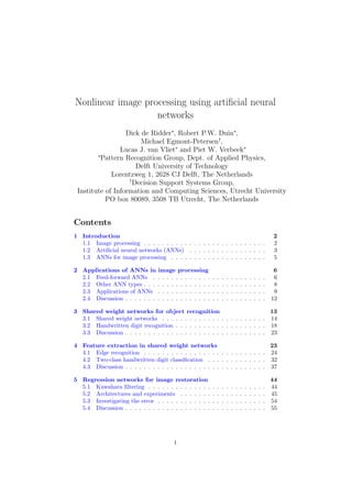
In figure 9, an image of the LeCun ANN trained on the entire training set
is shown. Some feature maps seem to perform operations similar to low-level
21
22. 20
18
16
14
12
10
8
6
4
2
0
0 200 400 600 800 1000
Training set size (samples/class)
Test set error (%)
nm
lc
qc
1nn
Figure 10: Performance of various classifiers trained on data sets extracted from
the feature extraction parts of the LeCun ANN.
image processing operators such as edge detection. It is also noteworthy that the
extracted features, the outputs of the last subsampling layer, are nearly binary
(either high or low). However, visual inspection of the feature and subsampling
masks in the trained shared weight ANNs in general does not give much insight
into the features extracted. Gader et al. (Gader et al., 1995), in their work on
automatic target recognition, inspected trained feature maps and claimed they
were “... suggestive of a diagonal edge detector with a somewhat weak response”
and “... of a strong horizontal edge detector with some ability to detect corners
as well”; however, in our opinion these maps can be interpreted to perform any
of a number of image processing primitives. In the next section, a number of
simpler problems will be studied in order to learn about the feature extraction
process in shared weight ANNs.
Here, another approach is taken to investigate whether the shared weight
ANNs extract useful features: the features were used to train other classifiers.
First, the architecture was cut halfway, after the last layer of subsampling maps,
so that the first part could be viewed to perform feature extraction only. The
original training, testing and validation sets were then mapped onto the new
feature space by using each sample as input and finding the output of this first
part of the ANN. This reduced the number of features to 192. In experiments,
a number of classifiers were trained on this data set: the nearest mean linear
classifier (nm), the Bayes plug-in linear and quadratic classifier (lc and qc) and
the 1-nearest neighbour classifier (1nn). For the Bayes plug-in classifiers, the
estimate of the covariance matrix was regularised in the same way as before (9),
using r = s = 0.1. Figure 10 shows the results.
In all cases the 1-nearest neighbour classifier performed better than the clas-sification
parts of the ANNs themselves. The Bayes plug-in quadratic classifier
performed nearly as well as the ANN (compare figure 8 (a) to figure 10. Interest-ingly,
the LeCun ANN does not seem to use its 30 unit hidden layer to implement
a highly nonlinear classifier, as the difference between this ANN’s performance
and that of the Bayes plug-in quadratic classifier is very small. Clearly, for all
shared weight ANNs, most of the work is performed in the shared weight layers;
after the feature extraction stage, a quadratic classifier suffices to give good
classification performance.
22
23. Most traditional classifiers trained on the features extracted by the shared
weight ANNs perform better than those trained on the original feature set (fig-ure
8 (b)). This shows that the feature extraction process has been useful. In
all cases, the 1-nearest neighbour classifier performs best, even better than on
the original data set (1.7% vs. 1.8% error for 1,000 samples/class).
3.3 Discussion
A shared weight ANN architecture was implemented and applied to a handwrit-ten
digit recognition problem. Although some non-neural classifiers (such as the
1-nearest neighbour classifier and some support vector classifiers) perform bet-ter,
they do so at a larger computational cost. However, standard feed-forward
ANNs seem to perform as well as the shared weight ANNs and require the same
amount of computation. The LeCun ANN results obtained are comparable to
those found in the literature.
Unfortunately, it is very hard to judge visually what features the LeCun ANN
extracts. Therefore, it was tested on its feature extraction behaviour, by using
the output of the last subsampling map layer as a new data set in training a
number of traditional classifiers. The LeCun ANN indeed acts well as a feature
extractor, as these classifiers performed well; however, performance was in at
best only marginally better than that of the original ANN.
To gain a better understanding, either the problem will have to be simplified,
or the goal of classification will have to be changed. The first idea will be worked
out in the next section, in which simplified shared weight ANNs will be applied
to toy problems. The second idea will be discussed in sections 5 and 6, in which
feed-forward ANNs will be applied to image restoration (regression) instead of
feature extraction (classification).
4 Feature extraction in shared weight networks
This section investigates whether ANNs, in particular shared weight ANNs,
are capable of extracting “good” features from training data. In the previ-ous
section the criterion for deciding whether features were good was whether
traditional classifiers performed better on features extracted by ANNs. Here,
the question is whether sense can be made of the extracted features by in-terpretation
of the weight sets found. There is not much literature on this
subject, as authors tend to research the way in which ANNs work from their
own point of view, as tools to solve specific problems. Gorman and Se-jnowski
(Gorman and Sejnowski, 1988) inspect what kind of features are ex-tracted
in an ANN trained to recognise sonar profiles. Various other authors
have inspected the use of ANNs as feature extraction and selection tools,
e.g. (Egmont-Petersen et al., 1998b; Setiono and Liu, 1997), compared ANN
performance to known image processing techniques (Ciesielski et al., 1992) or
examined decision regions (Melnik and Pollack, 1998). Some effort has also
been invested in extracting (symbolic) rules from trained ANNs (Setiono, 1997;
Tickle et al., 1998) and in investigating the biological plausibility of ANNs
(e.g. Verschure, 1996).
An important subject in the experiments presented in this section will be the
influence of various design and training choices on the performance and feature
23
24. (a)
0.00 4
2
0
−2
−4
1.00
0.00
1.00
−4.00
1.00
0.00
1.00
0.00
(b)
8
7
6
5
4
3
2
1
0
Frequency (x)
p
Frequency (y)
0
−p−p p 0
(c)
Figure 11: (a) The edge samples in the edge data set. (b) The Laplacian edge
detector. (c) The magnitude of the frequency response of the Laplacian edge
detector.
extraction capabilities of shared weight ANNs. The handwritten digit exper-iment
showed that, although the LeCun ANN performed well, its complexity
and that of the data set made visual inspection of a trained ANN impossible.
For interpretation therefore it is necessary to bring both data set and ANN
complexity down to a bare minimum. Of course, many simple problems can be
created (de Ridder, 1996); here, two classification problems will be discussed:
edge recognition and simple two-class handwritten digit recognition.
4.1 Edge recognition
The problem of edge recognition is treated here as a classification problem: the
goal is to train an ANN to give high output for image samples containing edges
and low output for samples containing uniform regions. This makes it different
from edge detection, in which localisation of the edge in the sample is important
as well. A data set was constructed by drawing edges at 0, 15, . . . , 345 angles
in a 256×256 pixel binary image. These images were rescaled to 16×16 pixels
using bilinear interpolation. The pixel values were -1 for background and +1
for the foreground pixels; near the edges, intermediate values occurred due to
the interpolation. In total, 24 edge images were created. An equal number of
images just containing uniform regions of background (−1) or foreground (+1)
pixels were then added, giving a total of 48 samples. Figure 11 (a) shows the
edge samples in the data set.
The goal of this experiment is not to build an edge recogniser performing bet-ter
than traditional methods; it is to study how an ANN performs edge recog-nition.
Therefore, first a theoretically optimal ANN architecture and weight
set will be derived, based on a traditional image processing approach. Next,
starting from this architecture, a series of ANNs with an increasing number of
restrictions will be trained, based on experimental observations. In each trained
ANN, the weights will be inspected and compared to the calculated optimal set.
24
25. Hidden layer (p)
14 x 14
Output layer (q)
1
Input layer (o)
16 x 16
w
w
b
po
p b
qp
q
I f L
edge
uniform
f(.) S f(.)
Figure 12: A sufficient ANN architecture for edge recognition. Weights and
biases for hidden units are indicated by wpo and bp respectively. These are the
same for each unit. Each connection between the hidden layer and the output
layer has the same weight wqp and the output unit has a bias bq. Below the
ANN, the image processing operation is shown: convolution with the Laplacian
template fL, pixel-wise application of the sigmoid f(.), (weighted) summation
and another application of the sigmoid.
4.1.1 A sufficient network architecture
To implement edge recognition in a shared weight ANN, it should consist of at
least 3 layers (including the input layer). The input layer contains 16×16 units.
The 14×14 unit hidden layer will be connected to the input layer through a 3×3
weight receptive field, which should function as an edge recognition template.
The hidden layer should then, using bias, shift the high output of a detected
edge into the nonlinear part of the transfer function, as a means of thresholding.
Finally, a single output unit is needed to sum all outputs of the hidden layer
and rescale to the desired training targets. The architecture described here is
depicted in figure 12.
This approach consists of two different subtasks. First, the image is convolved
with a template (filter) which should give some high output values when an
edge is present and low output values overall for uniform regions. Second, the
output of this operation is (soft-)thresholded and summed, which is a nonlinear
neighbourhood operation. A simple summation of the convolved image (which
can easily be implemented in a feed-forward ANN) will not do. Since convolution
is a linear operation, for any template the sum of a convolved image will be equal
to the sum of the input image multiplied by the sum of the template. This means
that classification would be based on just the sum of the inputs, which (given
the presence of both uniform background and uniform foreground samples, with
sums smaller and larger than the sum of an edge image) is not possible. The
data set was constructed like this on purpose, to prevent the ANN from finding
trivial solutions.
As the goal is to detect edges irrespective of their orientation, a rotation-
25
26. invariant edge detector template is needed. The first order edge detectors known
from image processing literature (Pratt, 1991; Young et al., 1998) cannot be
combined into one linear rotation-invariant detector. However, the second order
Laplacian edge detector can be. The continuous Laplacian,
fL(I) = @2I
@x2 + @2I
@y2 (10)
can be approximated by the discrete linear detector shown in figure 11 (b). It is
a high-pass filter with a frequency response as shown in figure 11 (c). Note that
in well-sampled images only frequencies between −
2 and
2 can be expected to
occur, so the filters behaviour outside this range is not critical. The resulting
image processing operation is shown below the ANN in figure 12.
Using the Laplacian template, it is possible to calculate an optimal set of
weights for this ANN. Suppose the architecture just described is used, with
double sigmoid transfer functions. Reasonable choices for the training targets
then are t = 0.5 for samples containing an edge and t = −0.5 for samples
containing uniform regions. Let the 3 × 3 weight matrix (wpo in figure 12)
be set to the values specified by the Laplacian filter in figure 11 (b). Each
element of the bias vector of the units in the hidden layer, bp, can be set to e.g.
bp
opt = 1.0.
Given these weight settings, optimal values for the remaining weights can be
calculated. Note that since the DC component5 of the Laplacian filter is zero,
the input to the hidden units for samples containing uniform regions will be just
the bias, 1.0. As there are 14 × 14 units in the hidden layer, each having an
output of f(1) 0.4621, the sum of all outputs Op will be approximately 196 ·
0.4621 = 90.5750. Here f(·) is the double sigmoid transfer function introduced
earlier.
For images that do contain edges, the input to the hidden layer will look like
this:
-1 -1 -1 -1 -1 -1
-1 -1 -1 -1 -1 -1
-1 -1 -1 -1 -1 -1
1 1 1 1 1 1
1 1 1 1 1 1
1 1 1 1 1 1
0 1 0
1 -4 1
0 1 0
=
0 0 0 0
2 2 2 2
-2 -2 -2 -2
0 0 0 0
(11)
There are 14 × 14 = 196 units in the hidden layer. Therefore, the sum of the
output Op of that layer for a horizontal edge will be:
X
i
Op
i = 14f(2 + bp
opt) + 14f(−2 + bp
opt) + 168f(bp
opt)
= 14f(3) + 14f(−1) + 168f(1)
14 · 0.9051 + 14 · (−0.4621) + 168 · 0.4621 = 82.0278 (12)
These values can be used to find the wqp
opt and bq
opt necessary to reach the targets.
Using the inverse of the transfer function,
f(x) =
2
1 + e−x
− 1 = a ) f−1(a) = ln
1 + a
1 − a
= x, a 2 h−1, 1i (13)
5The response of the filter at frequency 0, or equivalently, the scaling in average pixel value
in the output image introduced by the filter.
26
27. the input to the output unit, Iq =
P
i Op
i wqp
i + bq =
P
i Op
i wqp
opt + bq
opt = 0,
should be equal to f−1(t), i.e.:
edge: t = 0.5 ) Iq = 1.0986
uniform: t = −0.5 ) Iq = −1.0986 (14)
This gives:
opt + bq
edge: 82.0278 wqp
opt = 1.0986
opt + bq
uniform: 90.5750 wqp
opt = −1.0986 (15)
Solving these equations gives wqp
opt = −0.2571 and bq
opt = 22.1880.
Note that the bias needed for the output unit is quite high, i.e. far away from
the usual weight initialisation range. However, the values calculated here are all
interdependent. For example, choosing lower values for wpo and bp
opt will lead
to lower required values for wqp
opt and bq
opt. This means there is not one single
optimal weight set for this ANN architecture, but a range.
4.1.2 Training
Starting from the sufficient architecture described above, a number of ANNs
were trained on the edge data set. The weights and biases of each of these
ANNs can be compared to the optimal set of parameters calculated above.
An important observation in all experiments was that as more restric-tions
were placed on the architecture, it became harder to train. There-fore,
in all experiments the conjugate gradient descent (CGD, Shewchuk, 1994;
Hertz et al., 1991; Press et al., 1992) training algorithm was used. This algo-rithm
is less prone to finding local minima or diverging than back-propagation,
as it uses a line minimisation technique to find the optimal step size in each iter-ation.
The method has only one parameter, the number of iterations for which
the directions should be kept conjugate to the previous ones. In all experiments,
this was set to 10.
Note that the property that makes CGD a good algorithm for avoiding local
minima also makes it less fit for ANN interpretation. Standard gradient descent
algorithms, such as back-propagation, will take small steps through the error
landscape, updating each weight proportionally to its magnitude. CGD, due
to the line minimisation involved, can take much larger steps. In general, the
danger is overtraining: instead of finding templates or feature detectors that are
generally applicable, the weights are adapted too much to the training set at
hand. In principle, overtraining could be prevented by using a validation set, as
was done in section 3. However, here the interest is in what feature detectors
are derived from the training set rather than obtaining good generalisation. The
goal actually is to adapt to the training data as well as possible. Furthermore,
the artificial edge data set was constructed specifically to contain all possible
edge orientations, so overtraining cannot occur. Therefore, no validation set
was used.
All weights and biases were initialised by setting them to a fixed value of
0.01, except where indicated otherwise6. Although one could argue that random
6Fixed initialisation is possible here because units are not fully connected. In fully con-nected
ANNs, fixed value initialisation would result in all weights staying equal throughout
training.
27
28. 2
0
−2
1.86
1.30
1.06
1.30
−1.47
−1.02
1.06
−1.02
−3.07
(a)
8
7
6
5
4
3
2
1
Frequency (x)
p
Frequency (y)
0
−p−p 0 p
(b)
0.5
0
−0.5
(c)
2
1
0
−1
−2
(d)
Figure 13: (a) The template and (b) the magnitude of its frequency response, (c)
hidden layer bias weights and (c) weights between the hidden layer and output
layer, as found in ANN1.
initialisation might lead to better results, for interpretation purposes it is best
to initialise the weights with small, equal values.
ANN1: The sufficient architecture The first ANN used the shared weight
mechanism to find wpo. The biases of the hidden layer, bp, and the weights
between hidden and output layer, wqp, were not shared. Note that this ANN
already is restricted, as receptive fields are used for the hidden layer instead
of full connectivity. However, interpreting weight sets of unrestricted, fully
connected ANNs is quite hard due to the excessive number of weights – there
would be a total of 50,569 weights and biases in such an ANN.
Training this first ANN did not present any problem; the MSE quickly
dropped, to 1 × 10⁻⁷ after 200 training cycles. However, the template weight
set found – shown in figures 13 (a) and (b) – does not correspond to a Laplacian
filter, but rather to a directed edge detector. The detector does have a zero
DC component. Noticeable is the information stored in the bias weights of the
hidden layer bp (figure 13 (c)) and the weights between the hidden layer and
the output layer, wqp (figure 13 (d)). Note that in figure 13 and other figures in
this section, individual weight values are plotted as grey values. This facilitates
interpretation of weight sets as feature detectors. Presentation using grey values
is similar to the use of Hinton diagrams (Hinton et al., 1984).
Inspection showed how this ANN solved the problem. In figure 14, the dif-ferent
processing steps in ANN classification are shown in detail for three input
samples (figure 14 (a)). First, the input sample is convolved with the template
(figure 14 (b)). This gives pixels on and around edges high values, i.e. highly
negative (-10.0) or highly positive (+10.0). After addition of the hidden layer
bias (figure 14 (c)), these values dominate the output. In contrast, for uniform
regions the bias itself is the only input of the hidden hidden layer units, with val-ues
approximately in the range [−1, 1]. The result of application of the transfer
function (figure 14 (d)) is that edges are widened, i.e. they become bars of pixels
with values +1.0 or -1.0. For uniform regions, the output contains just the two
pixels diagonally opposite at the centre, with significantly smaller values.
The most important region in these outputs is the centre. Multiplying this
region by the diagonal +/- weights in the centre and summing gives a very
small input to the output unit (figure 14 (e)); in other words, the weights cancel
the input. In contrast, as the diagonal -/+ pair of pixels obtained for uniform
28
29. 1
0.5
0
−0.5
−1
5
0
−5
10
5
0
−5
−10
1
0.5
0
−0.5
−1
2
1
0
−1
−2
1
0.5
0
−0.5
−1
5
0
−5
10
5
0
−5
−10
1
0.5
0
−0.5
−1
2
1
0
−1
−2
1
0.5
0
−0.5
−1
5
0
−5
10
5
0
−5
−10
1
0.5
0
−0.5
−1
2
1
0
−1
−2
1
0.5
0
−0.5
−1
(a)
5
0
−5
(b)
10
5
0
−5
−10
(c)
1
0.5
0
−0.5
−1
(d)
2
1
0
−1
−2
(e)
Figure 14: Stages in ANN1 processing, for three different input samples: (a)
the input sample; (b) the input convolved with the template; (c) the total input
to the hidden layer, including bias; (d) the output of the hidden layer and (e)
the output of the hidden layer multiplied by the weights between hidden and
output layer.
samples is multiplied by a diagonal pair of weights of the opposite sign, the
input to the output unit will be negative. Finally, the bias of the output unit
(not shown) shifts the input in order to obtain the desired target values t = 0.5
and t = −0.5.
This analysis shows that the weight set found is quite different from the
optimal one calculated in section 4.1.1. As all edges pass through the centre
of the image, the edge detector need not be translation-invariant: information
on where edges occur is coded in both the hidden layer bias and the weights
between the hidden layer and the output layer.
ANN2: Sharing more weights To prevent the ANN from coding place-specific
information in biases and weights, the architecture will have to be sim-plified
further. As a restriction, in the next ANN architecture the weights
between the hidden layer and output layer were shared. That is, there was one
single weight shared among all 196 connections between the hidden units and
the output unit. Training took more time, but converged to a 1 × 10⁻⁶ MSE
29
30. 5
0
−5
4.05
0.51
−7.87
0.51
5.92
0.16
−7.87
0.16
4.42
(a)
30
25
20
15
10
5
Frequency (x)
p
Frequency (y)
0
−p−p 0 p
(b)
5
0
−5
(c)
Figure 15: (a) The template, (b) the magnitude of its frequency response and
(b) hidden layer bias weights as found in ANN2.
after 2,400 cycles. Still, the network does not find a Laplacian; however, the
template found (figure 15 (a) and (b)) has a more clear function than the one
found before. It is a strong detector for edges with slope −45, and a weak
detector for edges with slope 45.
In the bias weights of the hidden layer (figure 15 (c)), place-specific informa-tion
is now stored for edges which are not amplified well by this detector. Bias
weight values are also significantly higher than before (an average of -1.2144).
This allows the ANN to use the transfer function as a threshold operation, by
scaling large positive pixel values differently from large negative pixel values.
In conclusion, responsibility for edge recognition is now shared between the
template and the bias weights of the hidden layer.
ANN3: Sharing bias As the biases of hidden layer units are still used for
storing place-dependent information, in the next architecture these biases were
shared too7. Training became even harder; the ANN would not converge using
the initialisation used before, so weights were initialised to a fixed value of 0.1.
After 1,000 episodes, the MSE reached 8 × 10⁻⁴, just slightly higher than the
minimal error possible (at 3 × 10⁻⁴, larger than zero due to the interpolation
used in scaling the edge samples). The template found is shown in figures 16 (a)
and (b).
Note that the template now looks like a Laplacian edge
detector; its frequency
response is similar to that of the Laplacian in the range
−
2 ,
2
. However, there
are still small differences between various weights which are equal in the true
Laplacian. In fact, the filter seems to be slightly tilted, with the top left corner
containing weights with higher magnitude. Also, the frequency response shows
that the filter gives a bandpass response in diagonal directions. To obtain a
more Laplacian-like template, further restrictions will have to be placed on the
ANN.
ANN4: Enforcing symmetry In the last ANN, the prior knowledge that
the goal is to obtain a rotation-invariant filter was used as well, by sharing
7Sharing biases would have required a major rewrite of the simulation package used,
SPRLIB/ANNLIB (Hoekstra et al., 1996). Therefore, biases were shared by replacing all
biases by their average after each training cycle.
30
31. 2.33 4
2
0
−2
−4
−1.15
2.28
−1.15
−4.70
−1.06
2.28
−1.06
2.24
(a)
12
10
8
6
4
2
Frequency (x)
p
Frequency (y)
0
−p−p p 0
(b)
5
0
−5
−6.06
6.70
−6.06
6.70
−2.56
6.70
−6.06
6.70
−6.06
(c)
50
40
30
20
10
Frequency (x)
p
Frequency (y)
0
−p−p p 0
(d)
Figure 16: (a) The template found in ANN3 and (b) the magnitude of its
frequency response. (c) The template found in ANN4 and (d) the magnitude of
its frequency response.
weights in the filter itself. The mask used for this purpose was:
A B A
B C B
A B A
(16)
i.e. connections with identical mask letters used shared weights. Note that in
this ANN there are only 6 free parameters left: the three weights in the mask,
a bias weight for both the hidden and output layer and one weight between the
hidden and output layer.
Training was again more cumbersome, but after initialising weights with a
fixed value of 0.1 the ANN converged after 1,000 episodes to an MSE of 3×10⁻⁴.
The filter found is shown in figures 16 (c) and (d). Finally, a solution similar to
the optimal one
was found: its frequency response is like that of the Laplacian
in the range
−
2 ,
2
and the weights are symmetric.
4.1.3 Discussion
The experiments described in this section show that ANNs can be used as
edge detectors. However, the presence of receptive fields in the architecture in
itself does not guarantee that shift-invariant feature detectors will be found,
as claimed by some (Le Cun et al., 1990; Le Cun et al., 1989b; Viennet, 1993).
Also, the mere fact that performance is good (i.e., the MSE is low) does not
imply that such a feature extraction process is used. An important observation
in ANN1 and ANN2 was that the ANN will use weights and biases in later
layers to store place-dependent information. In such a network, where edge
positions are stored, in principle any template will suffice. Obviously, this makes
interpretation of these templates dubious: different observers may find the ANN
has learned different templates. One reason for the ease with which ANNs store
place-dependent information might be the relative simplicity of the dataset: the
fact that edges all passed through the centre of the image makes this possible.
Therefore, in the next section similar ANNs will be trained on a real-world
dataset.
When the ANNs were further restricted by sharing biases and other weights
(ANN3), convergence became a problem. The explanation for this is that the
31
32. Figure 17: The two-class handwritten digit data set.
optimal weight set is rather special in ANN terms, as the template has to have
a zero DC component (i.e., its weights have to add up to zero). Although
this seems to be a trivial demand, it has quite large consequences for ANN
training. Optimal solutions correspond to a range of interdependent weights,
which will result in long, narrow valleys in the MSE “landscape”. A small
perturbation in one of the template weights will have large consequences for the
MSE. Simple gradient descent algorithms such as back-propagation will fail to
find these valleys, so the line-optimisation step used by CGD becomes crucial.
The last ANN, ANN4, was able to find an edge detector very similar to the
Laplacian. However, this architecture was restricted to such an extent that it
can hardly be seen as representative for practical application of ANNs. This
indicates there is a trade-off between complexity and the extent to which ex-periments
are true-to-life on the one hand, and the possibility of interpretation
on the other. This effect might be referred to as a kind of ANN interpretability
trade-off 8. If an unrestricted ANN is trained on a real-world data set, the setup
most closely resembles the application of ANNs in everyday practice. However,
the subtleties of the data set and the many degrees of freedom in the ANN
prevent gaining a deeper insight into the operation of the ANN. On the other
side, once an ANN is restrained, e.g. by sharing or removing weights, lowering
the number of degrees of freedom or constructing architectures only specifically
applicable to the problem at hand, the situation is no longer a typical one. The
ANN may even become too constrained to learn the task at hand. The same
holds for editing a data set to influence its statistics or to enhance more prefer-able
features with regard to ANN training, which will be discussed in section 6.
4.2 Two-class handwritten digit classification
To construct a more real-life dataset while still maintaining the expectation
that weights can be interpreted, experiments with a small NIST subset were
performed. This subset consisted of 10 samples each of the classes “1” and “7”,
shown in figure 17. The 16 × 16 pixel values were scaled linearly between −1.0
(background) and 1.0 (foreground). Training targets were set to t = 0.5 for
class “1” and t = −0.5 for class “7”.
For this problem, it is already impossible to find an architecture and weight
set by hand which will give minimal error. The receptive fields in the ANNs are
8Note that this is not precisely the same issue as addressed by the bias-variance trade-off
(see page 8), which is concerned with the relation between model complexity and error.
The concern here is with the specificity of the model with respect to interpretation which, in
principle, is unrelated to complexity: making a model more specific need not introduce a bias.
32
33. expected to act as feature detectors, extracting characteristic shapes from the
data. Beforehand, it is quite hard to indicate by hand which weight sets will
detect the most salient features. However, as the width of the strokes in the
digit images lies in the range 3 − 5 pixels, feature detectors should have widths
and heights roughly in the range 3 − 7 pixels.
The starting point therefore will be the ANN used for edge recognition, shown
in figure 12. However, three different architectures will be used. The first has
a 3 × 3 pixel receptive field and 14 × 14 = 196 units in the hidden layer, the
second contains a 5×5 pixel receptive field and 12×12 = 144 hidden units and
the last contains a 7 × 7 pixel receptive field and 10 × 10 = 100 hidden units.
As for this data set it is to be expected that using more than one feature map
will increase performance, architectures using two feature maps were trained as
well. In this case, the number of hidden units doubles.
4.2.1 Training
Most ANNs were rather hard to train, again due to the restrictions placed on
the architecture. CGD was used with 10 steps during which directions were
kept conjugate. All ANN weights and biases were initialised using a fixed value
of 0.01, except where indicated otherwise. For most restricted architectures,
reaching an MSE of exactly 0 proved to be impossible. Therefore, training was
stopped when the MSE reached a sufficiently low value, 1.0 × 10⁻⁶.
ANN1: Unrestricted The first ANNs were identical to the one shown in
figure 12, except for the fact that three different ANNs were trained with 3 × 3
(ANN3×3
1 ), 5 × 5 (ANN5×5
1 ) and 7 × 7 (ANN7×7
1 ) pixel receptive fields, respec-tively.
These ANNs quickly converged to a nearly zero MSE: after 250 training
cycles, the MSE was in the order of 1 × 10⁻¹⁰. The feature detectors found,
shown in figure 18 (a), are not very clear however. The frequency responses
(figure 18 (b)) give more information. The filters most closely resemble horizon-tal
edge detectors: note the basic shape returning for the three sizes of feature
detector.
As was the case in the edge recognition ANNs, the weights between the hid-den
layer and the output unit have been used to store positions of the digits.
Figure 18 (c) illustrates this. Positive weights indicate pixel positions where
typically only class “7” samples have high values; negative weights indicate po-sitions
where class “1” is present. Although noisy, these same basic shapes are
present for each size of the receptive field.
In contrast to what was found for the edge recognition ANNs, the bias weights
in the second layer were not used heavily. Bias values fell roughly in the range
−2 × 10⁻², 2 × 10⁻²
, i.e. negligible in comparison to feature detector weight
values.
ANN2: Fully restricted In the next architecture, the number of weights
was restricted by sharing weights between hidden layer and output layer and by
sharing the bias weights in the second layer (i.e., the basic architecture was the
same as ANN3 for edge recognition, on page 30). As a consequence, there were
far fewer parameters left in the ANNs: the number of weights in the feature
detector plus two biases and one weight between hidden and output layer.
Training became quite a bit harder. It did not converge for the ANN with the
3 × 3 pixel receptive field; the MSE oscillated around 1.5 × 10⁻². For the other
two ANNs, training was stopped when the MSE fell below 1×10⁻⁶, which took
33
34. 2000 cycles for the 5×5 pixel receptive field ANN and 1450 cycles for the 7×7
pixel receptive field ANN.
The feature detectors found are shown in figure 19. Note that since the 3×3
receptive field ANN did not converge, the resulting filter cannot be interpreted.
Since the weights between hidden layer and output layer can no longer be used,
the feature detectors of the other two look rather different. The 5 × 5 pixel
feature detector is the most pronounced: it is a detector of 3-pixel wide bars
with a slope of 45. Evidence for this can also be found by inspecting the output
of the hidden layer for various inputs, as shown in figure 20. In the location of
the stem of the “7”s, output values are much higher than those in the location
of the stem of the “1”s. Finally, the function of the 7 × 7 pixel feature detector
is unclear.
From these results, it is clear that a feature detector size of 3×3 pixels is too
small. On the other hand, although the 7 × 7 pixel feature detector gives good
performance, it cannot be interpreted well. The 5 × 5 pixel feature detector
seems to be optimal. Therefore, from here on only 5 × 5 pixel feature detectors
will be considered.
ANN3: Two feature maps Although the frequency response of the 5 × 5
pixel feature detector is clearer than the others, the filter itself is still noisy, i.e.
neighbouring weights have quite different values. There is no clear global feature
(within a 5 × 5 pixel region) that corresponds to this detector. The reason
for this might be that in fact several features are detected (either amplified
or attenuated) using this one set of weights. Therefore, ANN3 contained two
feature maps instead of one. In all other respects, the ANN was the same as
ANN5×5
2 , as shown in figure 21.
If this ANN is initialised using a fixed value, the two feature detectors will
always remain identical, as each corresponding weight in the two detectors is
equally responsible for the error the ANN makes. Therefore, random initialisa-tion
is necessary. This frustrates interpretation, as different initialisations will
lead to different final weight sets. To illustrate this, four ANNs were trained in
which weights were initialised using values drawn from a uniform distribution
with range [−0.01, 0.01]. Figure 22 shows four resulting template pairs. The
feature detector found before in ANN5×5
2 (figure 19) often returns as one of the
two feature maps. The other feature detector however shows far more variation.
The instantiation in the second row of figure 22 (b) looks like the horizontal
edge detector found in ANN1 (figures 18 (a), (b)), especially when looking at its
frequency response (in the fourth column). However, in other ANNs this shape
does not return. The first and fourth ANN indicate that actually multiple fea-ture
detectors may be distributed over the two feature maps.
To allow inspection of weights, initialisation with fixed values seems to be a
prerequisite. To allow this, the training algorithm itself should allow initially
identical weights to take on different values during training. The next section
will introduce a training algorithm developed specifically for training ANNs with
the goal of weight interpretation.
4.2.2 Decorrelating conjugate gradient descent
The last experiment on the NIST subset showed that interpretation of ANNs
with multiple feature detectors is difficult. The main causes are the random
weight initialisation required and a tendency of the ANNs to distribute features
34
35. to be detected in a non-obvious way over receptive fields. To address the latter
problem, hidden units learning identical functions, a modular approach has been
suggested (Jacobs et al., 1991). However, this is not applicable in cases in which
there is no clear decomposition of a task’s input space into several domains.
To allow fixed value weight initialisation and still obtain succinct feature
detectors, a new training algorithm will be proposed. The algorithm is based
on CGD, but has as a soft constraint the minimisation of the squared covariance
between receptive fields. In this way, the symmetry between feature detectors
due to fixed value initialisation can be broken, and receptive field weight sets
are forced to become orthogonal while still minimising the ANN’s MSE.
Decorrelation Note that, in trained ANNs, weight sets belonging to different
receptive fields need not be exactly the same for the feature maps to perform the
same function. This is because weights are interdependent, as was already noted
in section 4.1.1. As an example, consider the weight vectors wpo,A and wpo,B
(from here on, wA and wB) in ANN3 (figure 21). As long as wA = c1wB + c2,
biases in the hidden and output layer and the weights between these layers can
correct the differences between the two weight sets, and their functionality can
be approximately identical9. The conclusion is that to compare weight sets, one
has to look at their correlation.
Suppose that for a certain layer in an ANN (as in figure 21) there are two
incoming weight vectors wA and wB, both with K 2 elements and var(wA)
0 and var(wB) 0. The correlation coefficient C between these vectors can be
calculated as:
C(wA,wB) =
cov(wA,wB)
p
var(wA)var(wB)
(17)
The correlation coefficient C(wA,wB) is a number in the range [−1, 1]. For
C(wA,wB) = ±1, there is a strong correlation; for C(wA,wB) = 0 there is no
correlation. Therefore, the squared correlation C(wA,wB)2 can be minimised
to minimise the likeness of the two weight sets.
Although this seems a natural thing to do, a problem is that squared cor-relation
can be minimised either by minimising the squared covariance or by
maximising the variance of either weight vector. The latter is undesirable, as
for interpretation the variance of one of the weight vectors should not be un-necessarily
increased just to lower the squared correlation. Ideally, both weight
vectors should have comparable variance. Therefore, a better measure to min-imise
is just the squared covariance. To do this, the derivative of the covariance
w.r.t. a single weight wAi
has to be computed:
@cov(wA,wB)2
@wAi
= @
@wAi
1
K
PK
k=1(wAk
− wA)(wBk
2
− wB)
=
2
K
cov(wA,wB)(wBi
− wB) (18)
This derivative can then be used in combination with the derivative of the MSE
w.r.t. the weights to obtain a training algorithm minimising both MSE and
squared covariance (and therefore squared correlation, because the variance of
9Up to a point, naturally, due to the nonlinearity of the transfer functions in the hidden
and output layer. For this discussion it is assumed the network operates in that part of the
transfer function which is still reasonably linear.
35
36. the weight vectors will remain bounded since the ANN still has to minimise the
MSE).
Correlation has been used before in neural network training. In the cascade
correlation algorithm (Fahlman and Lebiere, 1990), it is used as a tool to find
an optimal number of hidden units by taking the correlation between a hidden
unit’s output and the error criterion into account. However, it has not yet been
applied on weights themselves, to force hidden units to learn different functions
during training.
A decorrelating training algorithm Squared covariance minimisation was
incorporated into the CGD method used before. Basically, CGD iteratively
applies three stages:
• calculation of the derivative of the error w.r.t. the weights, dE = @
@wE(w);
• deriving a direction h from dE which is conjugate to previously taken
directions;
• a line minimisation of E from w along h to find a new weight vector w0.
The squared covariance term was integrated into the derivative of the error
function as an additive criterion, as in weight regularisation (Bishop, 1995). A
problem is how the added term should be weighted (cf. choosing the regularisa-tion
parameter). The MSE can start very high but usually drops rapidly. The
squared covariance part also falls in the range [0,1i, but it may well be the
case that it cannot be completely brought down to zero, or only at a significant
cost to the error. The latter effect should be avoided: the main training goal is
to reach an optimal solution in the MSE sense. Therefore, the covariance infor-mation
is used in the derivative function only, not in the line minimisation. The
squared covariance gradient, dcov, is normalised to the length of the ordinary
gradient dE (just its direction is used) and weighed with a factor ; i.e. d =
dE + ||dE||
||dcov||dcov, where dcov = 2
K(K−1)
PK−1
k=1
PK
l=k+1
@
@wcov(wk(0),wl(0))2.
Note that the derivative of the squared covariance is only calculated once for
each pair of weight sets and attributed to only one of the weight sets. This allows
one weight set to learn a globally optimal function, while the second set is trained
to both lower the error and avoid covariance with the first set. It also allows ini-tialisation
with fixed values, since the asymmetrical contribution of the squared
covariance term provides a symmetry breaking mechanism (which can even im-prove
performance in some classification problems, see de Ridder et al., 1999).
However, the outcome of the DCGD training process is still dependent on the
choice of a number of parameters. DCGD even introduces a new one (the weight
factor ). If the parameters are chosen poorly, one will still not obtain under-standable
feature detectors. This is a problem of ANNs in general, which cannot
be solved easily: a certain amount of operator skill in training ANNs is a pre-requisite
for obtaining good results. Furthermore, experiments with DCGD are
reproducable due to the possibility of weight initialisation with fixed values.
The DCGD algorithm is computationally expensive, as it takes covariances
between all pairs of receptive fields into account. Due to this O(n2) complexity
in the number of receptive fields, application of this technique to large ANNs
is not feasible. A possible way to solve this problem would be to take only a
subset of covariances into account.
36
37. 4.2.3 Training ANN3 using DCGD
ANN3 was trained using DCGD. Weights and biases were initialised to a fixed
value of 0.01 (i.e. μ = 0.01, = 0.0) and N = 10 directions were kept conjugate
at a time. The only parameter varied was the weighting factor of the squared
covariance gradient, , which was set to 0.5, 1, 2 and 5. Training converged
but was slow. The MSE eventually reached the values obtained using CGD
(1.0 × 10⁻⁶, cf. section 4.2.1); however, DCGD training was stopped when
the MSE reached about 1.0 × 10⁻⁵, after about 500-1000 cycles, to prevent
overtraining. In all cases, classification was perfect.
Figure 23 shows the feature detectors found in ANN3 trained using DCGD.
Squared correlations C2 between them are very small, showing that the min-imisation
was succesful (the squared covariance was, in all cases, nearly 0). For
= 1 and = 2, the feature detectors are more clear than those found using
standard CGD, in section 44.24.2.1 Their frequency responses resemble those of
the feature detectors shown in figure 22 (b) and, due to the fixed weight initiali-sation,
are guaranteed to be found when training is repeated. However, should
be chosen with some care; if it is too small ( = 0.5), the squared covariance
term will have too little effect; if it is too large ( = 5), minimisation of the
squared covariance term becomes too important and the original functionality
of the network is no longer clearly visible.
The features detected seem to be diagonal bars, as seen before, and horizontal
edges. This is confirmed by inspecting the output of the two feature maps in
ANN3 trained with DCGD, = 1, for a number of input samples (see figure 24).
For samples of class “1”, these outputs are lower than for class “7”, i.e. features
specific for digits of class “7” have been found. Furthermore, the first feature
detector clearly enhances the stem of “7” digits, whereas the second detector
amplifies the top stroke.
Finally, versions of ANN3 with three and four feature maps were also trained
using DCGD. Besides the two feature detectors found before no clear new feature
detectors were found.
4.3 Discussion
The experiments in this section were performed to find whether training ANNs
with receptive field mechanisms leads to the ANN finding useful, shift-invariant
features and if a human observer could interpret these features. In general, it
was shown that the mere presence of receptive fields in an ANN and a good
performance do not mean that shift-invariant features are detected. Interpreta-tion
was only possible after severely restricting the ANN architecture, data set
complexity and training method.
One thing all experiments had in common was the use of ANNs as classifiers.
Classification is a “derived” goal, i.e. the task is assigning (in principle arbi-trary)
outputs, representing class labels, to input samples. The ANN is free to
choose which features to use (or not) to reach this goal. Therefore, to study the
way in which ANNs solve problems moving to regression problems might yield
results more fit for interpretation, especially when a regression problem can be
decomposed into a number of independent subproblems. The next sections will
study the use of ANNs as nonlinear filters for image enhancement.
37