1. Weibull Analysis
The Weibull distribution is one of the most commonly used distributions in Reliability
Engineering because of the many shapes it attains for various values of β. Weibull analysis
continues to gain in popularity for reliability work, particularly in the area of mechanical
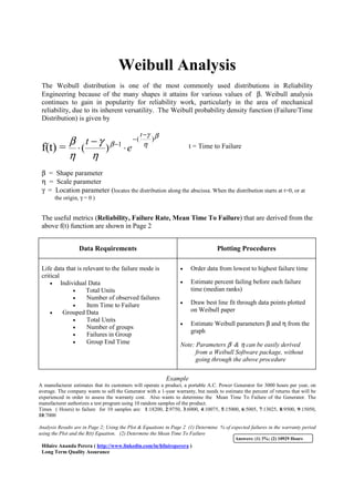
reliability, due to its inherent versatility. The Weibull probability density function (Failure/Time
Distribution) is given by
t −γ β
β t − γ β −1 − ( η
)
f(t) = ⋅ ( ) ⋅e t = Time to Failure
η η
β = Shape parameter
η = Scale parameter
γ = Location parameter (locates the distribution along the abscissa. When the distribution starts at t=0, or at
the origin, γ = 0 )
The useful metrics (Reliability, Failure Rate, Mean Time To Failure) that are derived from the
above f(t) function are shown in Page 2
Data Requirements Plotting Procedures
Life data that is relevant to the failure mode is • Order data from lowest to highest failure time
critical
• Individual Data • Estimate percent failing before each failure
• Total Units time (median ranks)
• Number of observed failures
• Draw best line fit through data points plotted
• Item Time to Failure
• Grouped Data on Weibull paper
• Total Units
• Estimate Weibull parameters β and η from the
• Number of groups
graph
• Failures in Group
• Group End Time Note: Parameters β & η can be easily derived
from a Weibull Software package, without
going through the above procedure
Example
A manufacturer estimates that its customers will operate a product, a portable A.C. Power Generator for 3000 hours per year, on
average. The company wants to sell the Generator with a 1-year warranty, but needs to estimate the percent of returns that will be
experienced in order to assess the warranty cost. Also wants to determine the Mean Time To Failure of the Generator. The
manufacturer authorizes a test program using 10 random samples of the product.
Times ( Hours) to failure for 10 samples are: 1:18200, 2:9750, 3:6000, 4:10075, 5:15000, 6:5005, 7:13025, 8:9500, 9:15050,
10:7000
Analysis Results are in Page 2; Using the Plot & Equations in Page 2 (1) Determine % of expected failures in the warranty period
using the Plot and the R(t) Equation. (2) Determine the Mean Time To Failure
Answers: (1) 3%; (2) 10929 Hours
Hilaire Ananda Perera ( http://www.linkedin.com/in/hilaireperera )
Long Term Quality Assurance

2. Use Of Weibull Analysis
β = 2.58
Q(t) = Probability of Failure as a percentage η = 12310 Hours
t
−( ) β β = Shape Parameter
η
Reliability Function R(t) = e η = Scale Parameter
β t β −1
t = Operating Time
Failure Rate Function λ(t) = ( ) Γ( β -1 +1) is the Gamma
η η Function evaluated at the
value of (β -1 +1)
1
Mean Time To Failure m = ηΓ ( + 1)
β
NOTE: Mean Time To Failure is the inverse of Failure Rate only when β = 1
Hilaire Ananda Perera ( http://www.linkedin.com/in/hilaireperera )
Long Term Quality Assurance

3. Interpreting The Weibull Plot
Value of β Product If this occurs, suspect the following
Characteristics
β<1 Implies infant • Inadequate stress screening or Burn-In
mortality. If • Quality problems in components
product survives • Quality problems in manufacturing
infant mortality, its • Rework/refurbishment problems
resistance to failure
improves with age
β=1 Implies failures are • Maintenance/human errors
random. An old • Failures are inherent, not induced
part is just as good • Mixture of failure modes
(or bad) as a new
part
β>1&<4 Implies early • Low cycle fatigue
wearout • Corrosion or erosion failure modes
• Scheduled replacement may be cost effective
β>4 Implies old age • Inherent material property limitations
(rapid) wearout • Gross manufacturing process problems
• Small variability in manufacturing or material
Ref: RAC Reliability Toolkit
Hilaire Ananda Perera ( http://www.linkedin.com/in/hilaireperera )
Long Term Quality Assurance