1. MARKET ULTIMATE PROFITABILITY1
Alexei KAZAKOV* and Maria PLOTNIKOVA**
Abstract. In this article a problem of market research effectiveness is raised
and a method to evaluate it is proposed. The authors introduce a concept of
ultimate profitability of any particular market instrument or index. Syste-
matic time shifts in market position changes from an ideal timing are consi-
dered as a reason of actual profitability declining from ultimate one and are
suggested to serve as a measure of market research effectiveness. The
ultimate profitability concept itself turns up to be a fruitful one able to
reinforce comparative studies of national markets and market tools, invest-
ment styles and volatility studies. Following observations of emerging equity
markets ultimate profitability characteristics the phenomena of hyper
volatility is revealed and a clue to a rationale of high frequency long-short
trading are received.
Keywords: market, investments, research, profitability, volatility.
1. Introduction
Economy of portfolio investments
Portfolio investments theory is much about balancing expected return
with risk of a desired level. Given that risk is fixed at certain level each
portfolio investor strives to enhance yield of investments. In practice the
choice is limited: either to increase the gross results of investment activity
or to decrease the operating costs, associated with it. It is possible to try to
move simultaneously in both directions, but at some moment an increase in
a result and reduction in expenditures may start contradicting each other. In
particular, so it occurs, if one economizes on research and/or market data
processing.
If an investor plans to maintain some level of expenditures on
analytical support, then there is a question: whether it is possible to
*1
Occupations as of year 2005 start when the study was conducted.
**
Allianz ROSNO Aseet Management, Post address: Ramenki st., 7/2/351,
Moscow, Russian Federation, 119607, e-mail: alexei.e.kazakov@gmail.com.
**
Uralsib Capital, Post address: Rozenlaan 2a bus 11702 Groot-Bijgaarden,
Belgium, e-mail: marpl7@yahoo.com.
69

2. introduce any criterion for effectiveness of those expenditures? In case
an investor is institutional that may be a question of a sizable economic
significance.
2. Ideal timing, or the hypothesis about zero shift
Unlike the majority of other costs, which accompany operations on
financial markets, expenditures on research – is a rather poorly defined
concept, and these costs are subjected to testing on the effectiveness with
difficulty. We attempt to estimate the contribution of analytical support to
the determination of the optimum moment of changing the market position.
To the market participants this process is well known as a choice of right
time to enter the market or, in short, the timing. Much of real life
investment analytical cases can be transformed / reduced into the form of
timing problem.
Let’s accept for an axiom, that the best moments for changing market
position are those ones when prices achieve their local extremes – local
maximum or minimum values. Let’s imagine that someone can syste-
matically determine these price extremes with ideal preciseness. And let’s
call this assumption “the hypothesis about zero shift”. In practice things are
not so bright: with poor analytical advice an investor risks to take market
position far from right moment and/or even not in right direction (which
can also be considered as a significant error in a choice of ‘right time’). It
is almost self-evident that any actual timing process includes non-zero
shifts. A well informed practitioner will tend to make relatively small
shifts, while his less prepared competitor will make systematically larger
shifts. We’ll consider the average (‘systematic’) proximity of real timing to
the ideal one as a criterion of analytical support quality.
3. Market ultimate profitability
3.1. Working Hypothesis
To measure the economic effect of shifts we need to evaluate the
dependence of investment return on systematic shifts. The sequence of
study asserts by itself: the history of some market tool prices is taken for
few years and all extreme lows and highs are determined (points of turn on
the price graph). Taking into account this marking it is defined ultimate –
70

3. maximally possible – annual profitability of active investment operations
with that market tool, and then it is fixed how this theoretical profitability
changes with an increase in a systematic shift of ‘actual’ moments of
market position turn (from Long to Short and vice versa) from ‘ideal’ local
price extremes. We assume that trading can be done in both directions (up
and down) symmetrically easy (i.e. terms for both Buy and Sell Short
orders execution are equal).
There is, perhaps, only one problem with this approach: it is possible
to reveal multiple extremes of different scale on the price graph. Therefore
before taking up the measurement of ultimate profitability, it is necessary
to agree about the extent of detailing, needed for studying the price
behavior. From mathematical point of view this problem resembles the
coastline paradox2, popularized by Benoit Mandelbrot [1]. Thus, we
address self-similarity in price behavior by fixing the scale of price move-
ments from one extreme to another. Also for the purposes of this study it is
more convenient to use percentage measurement of price increments
(whereas in fractal studies logarithms are used more often).
After all these assumptions and stipulations have been done we can
give clearer definition of what market ultimate profitability is. Average
annual ultimate profitability calculated for a number of years shows how
much a capital invested in a particular market tool would cumulatively
grow in one year (in %) on average, with an assumption that an investor
occupies alternately long and short market positions, changing them
accurately at the price extremes, which are distant to each other not less
than the predetermined value N (in % of entry price). Value N in fact
serves similar to a linear measure when determining the distance (in %)
overcame by a particular market tool price (remember ‘coastline paradox’).
While measuring price movements (from one extreme to another) we
‘don’t notice’ movements less than N. A particular measured movement
can be, however, much bigger that N (depending on market dynamics).
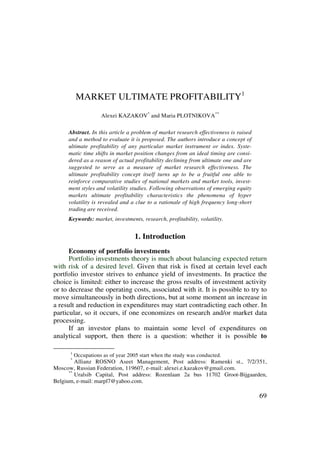
Ultimate profitability should grow with decreasing N as ‘market distance’
traveled by price increases. In figure 1 the dependence of average annual
2
The length of coastline depends on a minimum increment of ‘yard-measure’. The
smaller the increment, the longer the coastline occurred. A study of this paradox gave
start to much of Benoit Mandelbrot’s later work which led to an introduction in 1975 of a
new term: fractal. Fractals is a numerous class of mathematical objects, describing many
natural forms, for instance, surfaces of woods and corals as well as graphs of market
prices [2,3,4].
71

4. ultimate profitability on value N is presented, calculated for Russian equity
RUIX index (December 1996-July 2004). Similar experimental curves can
be obtained for any tradable asset or market index.
100 000
%
Av erage annual ultimate profitability
(%, per annum)
10 000
y = 125190x -1.5072
R 2 = 0.9939
1 000
Variable N - minimal distance betw een
price rev ersal points (% of price)
%
100
0.5% 2.5% 4.5% 6.5% 8.5% 10.5% 12.5% 14.5% 16.5% 18.5%
Figure 1. Dependence of average annual ultimate profitability (%)
on variable N (%). RUIX index.
Source: RTS.
Note. While being an artificial construct created for the purposes of
this study the average annual ultimate profitability by its economic sense is
very close to the return on capital (ROC, a concept widely used in
business). It perfectly represents market dynamics and helps to reveal the
role of timing. It does not represent, however, some practical aspects /
components affecting yield of tradable financial/commodity instruments:
dividend (for equities), accrued interest (for bonds and notes), leverage (for
futures and options), strike price (for options) and various built-in terms
(for structured products). If necessary (not for the purposes of this study)
ultimate profitability can be adjusted for those yield components / aspects.
72

5. 3.2. Choice of Scale
Before fixing the scale of market consideration let’s examine the
dependence of an average annual ultimate profitability and number of
market position reversals (transactions) on parameter N, % based on the
Russian equity index RTS (Fig. 2).
30 Average annual number Ultimate 5 000
of reversals (trades) profitability,% %
25
4 000
RTSI 15 - av erage number of rev ersals per annum (1995-2004)
RTSI 15 - av erage number of rev ersals per annum (1999-2004)
20
RTSI - av erage ultimate profitability (1995-2004)
3 000
RTSI - av erage ultimate profitability (1999-2004)
15
2 000
10
1 000
5
Variable N - minimal distance betw een
price rev ersal points (% of price)
0 0
5 10 15 20 25 N,% 30
Figure 2. Dependence of the average annual number of market position reversals
and ultimate profitability on the variable N (%). RTS index.
Source: RTS.
The obtained curves show that the less is N, the more turns the
investor has to perform and the higher theoretically possible investment
return (ultimate profitability), and vice versa. In practice a decrease in N is
limited with market liquidity and trading costs. The types of available
market news/data analysis also provide certain restrictions. For instance,
from the practical observations on the Russian equity market the
macroeconomic analysis will be useful with N not less than 15-20%, the
analysis of corporate financial reports – with N in a range 10-15%. Only
those ready to play on news or to exploit the technical analysis/statistical
73

6. methods, can withstand moderate equity market fluctuations (N < 10%).
Typical research department performs types of analysis listed above which
gives us N =15% on balance. Interestingly enough that, as it follows from
figure 2, under active management of an index portfolio (which copies the
composition of RTS or RUIX indices), it is theoretically possible to obtain
on Russian equity market a 3-digit annual return, reversing market posi-
tions not more often than 5 times/year on average.
3.3. Results: Influence of Systematic Shift
Thus, the ultimate profitability, which theoretically can be achieved
under active management of investor’s portfolio, is the function of N, %3.
Variable N has a direct relevance to formulating the task for the analytical
support service, since different types of investment analysis are suitable to
analyze and forecast price changes of different scale. Let’s fix N at 15% to
make it closer to practice and move further.
The next step within this study is imposition of systematic shift into
the optimum ‘time-table’ of the market positions reversals. Regular
(systematic) delay from the optimum moments of changing the position,
for instance, on one day (+1d) would mean that the imaginary investor
always (systematically) is one day late and turns his market position one
day after prices have reached a local extreme. Systematic outrunning of
reversal points is also possible, let’s say, on 7 days (–7d). As seen on the
figure 3, the ‘shifted’ ultimate profitability rather rapidly and symmetri-
cally decreases with an increase in the systematic shift modulus (from 1 to
10 days). One of two curves on the figure 3 represents ‘shifted’ ultimate
profitability (N =15%) based on data set which includes year 1997 (Asian
crisis) and year 1998 (Russian crisis), another curve – on data which
doesn’t include those years. The spread between two of them gives an idea
to what extent financial shocks impact average ultimate profitability.
Both curves decline with an increase in systematic shift modulus – rapidly
near the zero shift locality and more slowly on more distant localize.
Knowing the value of assets under management, actual systematic shift
and curve’s differential (angle) allows anyone to calculate arithmetically
3
There is some experimental evidence that ultimate profitability is an inverse power
function of N (see Fig. 1).
74

7. whether higher expenses for research (to decrease systematic shift
from ideal timing) are justified with the expected increase of investment
return or not.
1 400
%
Ultimate profitability
1 200
RTSI 15 - average
ultimate profitability
1 000 (1999-2004)
RTSI 15 - average
800 ultimate profitability
(1995-2004)
600
400
200
Systematic shift, days
0
-10d' -8d' -6d' -4d' -2d' 0 +2d' +4d' +6d' +8d' +10d'
Figure 3. Dependence of ‘shifted’ ultimate profitability (N =15%),
% on a systematic shift (days). RTS index.
Source: RTS.
3.4. Active vs Passive Asset Management
In case a set up or a liquidation of research department is considered
one would better know not the effect from in-or de-crease of research
expenses but the basic interrelation of investment style, quality of analy-
tical support (expressed in terms of a systematic shift) and spending
on analytics. To make it possible let’s draw a few ‘shifted’ ultimate profita-
bility curves (for various N) on one graph together with a <horizontal> level
of an average return demonstrated by broad target market index (Fig. 4).
This horizontal line represents historical average annual return received by
passive investor. In practice it corresponds to return delivered by index
mutual fund. According to classics [5,6] multi-year periods have to be taken.
75

8. 10,000
"Buy & Hold" strategy
% RTSI 5
RTSI 10
Ultimate profitability
RTSI 15
RTSI 20
RTSI 25
RTSI 30
1,000
100
Systematic shift, days
10
-10d' -8d' -6d' -4d' -2d' 0 +2d' +4d' +6d' +8d' +10d'
Figure 4. ‘Shifted’ ultimate profitability curves for
various N, % (5%-30%). RTS index.
Source: RTS.
For short period of time there is a clear risk to get a negative reading.
As a sample Russian equity market is pretty young we have used just
5-years period (1999-2004) during which index RTS growth is appr. 50%
per annum on average. As it follows from figure 4, for an investor willing
to play market waves with an amplitude 10% and above it is important
to “catch” the extreme points of the index with an accuracy not worse than
+/–10 days (deviation from ideal timing). If expected or actual accuracy
(obtained from track records) is less favorable, it is better to follow
long-term passive strategy ‘Buy & Hold’, and to reduce research costs to
nil (or attribute them to marketing expenditures). In case an investor is
going to play smaller market waves (5%+), he needs to be in time to “turn
over” market position twice more rapidly, with an accuracy not worse
than +/–5 days for systematic shift. Otherwise results are worse than
if he/she follows strategy ‘Buy & Hold’. It is interesting that with more
measured investment strategies targeting at market 20-25-30% waves it
76

9. is possible to get more than 100% annual investment return (which is twice
bigger than ‘Buy & Hold’ strategy shows in Russia), – even with the
systematic oversight of 10 days to or past the date of the market reversals (of
chosen scale).
4. Ultimate profitability and volatility.
Hyper volatility
We think that ultimate profitability is closely linked to market volati-
4
lity . To distinguish ‘excessive’ market moves characteristic it is sufficient
to divide ultimate profitability by net directional move of the market during
the time period under consideration. This net directional move is a constant
(%) as it remains the same for all N indications within the chosen time
period (and shift equals zero). That means that ultimate profitability and
volatility are linked linearly. It might be very convenient in some cases as
it allows using ultimate profitability for estimates of both potential return
and potential risk (volatility).
Inter-market comparisons reveal yet another useful feature of ultimate
profitability curves. As it is seen on a chart above (Fig. 5) curves corres-
ponding to emerging markets [BUX – Hungary, MEXBOL – Mexico,
BOVESPA – Brazil, KOSPI – South Korea, RTSI – Russia, MSCI EMF –
composite MSCI index] are considerably higher than S&P500 index’s
curve. This is not a surprise as emerging equity markets are famous for
their volatility (in a comparison with matured markets). But what can be a
surprise is that Russian RTS index ‘shifted’ ultimate profitability is notably
higher than analogous curves for other emerging markets indices within the
range of +/–8 days shift. In our view this is a clear demonstration that some
emerging markets (incl. Russian and Chinese equity markets) can be even
more volatile than others in the group. Obviously, the hyper volatility of a
market increases the risk of passive investments in it, but at the same time
it represents a potential for an advanced active investor.
4
This and following parts of article were added, significantly or partially re-wor-
ked in 2010, while previous text was published earlier in Russian-language magazine
‘Securities Market’ in 2005 [7].
77

10. RTSI 15 - av erage ultimate profitability (1999-2004)
1 000 KOSPI 15
Ultimate profitability
% BOVESPA 15
MSCI EMF 15
MEXBOL 15
BUX 15
S&P500 15
100
Systematic shift, days
10
-10d' -8d' -6d' -4d' -2d' 0 +2d' +4d' +6d' +8d' +10d'
Figure 5. ‘Shifted’ ultimate profitability curves for
various national stock indices (N = 15%).
Source: Bloomberg, RTS.
5. Particularities of investing on emerging markets
Another findings, which can be made basing on a comparison of
ultimate profitability curves for various market instruments, relates to an
old and still ongoing discussion about different investment styles.
Popularity of emerging markets among international investors increa-
sed tremendously in last decades. The number of liquid instruments
available for big institutional investors on emerging markets remains,
however, insignificant. For instance, there is around a dozen of Russian
blue chips investable for big international equity investors. That means that
following a concept of highly diversified portfolio on emerging markets is
impossible. International investors’ portfolios – due to the limited choice
of investable liquid stocks – involuntarily consist mainly of a limited num-
ber of the same ‘blue chips’. Since many local ‘blue chips’ demonstrate
even higher volatility than that of market index (Fig. 3 and Fig. 6) the
portfolios consisting of them are subjected to market fluctuations with
accentuated magnitude. Thus, the natural way for an international investor
is to manage his/her portfolio actively and to play waves down.
78

11. Year 2008 was a disaster for local institutional investors on emerging
markets. In Russia most of pension funds’ and insurance companies’
portfolios were not prepared for market declines of such magnitude (~75%
in index RTS). Looking into the future, disappointment of institutional
investors can be a very costly thing for national markets development. So
learning lessons of year 2008 (Y08) is of critical importance for the future
of emerging markets. And one of those lessons is that passive investments
are not adequate strategy for a conservative investor bound to work on
highly volatile market. Another lesson is that emerging markets’ high
economic growth potential doesn’t mean that they are immune to external
financial shocks. All in all institutional investors from emerging markets
need investment strategies and respective financial products which more
adequately reflect the nature of their native local financial markets. We
believe that market ultimate profitability concept helps to reveal that nature
and to explain some of it specific features.
10 000
% LKOH 15
U ltim ate profitability
SBER 15
EESR 15
SNGS 15
RTKM 15
1 000 MSNG 15
100
Systematic shift, days
10
-10d' -8d' -6d' -4d' -2d' 0 +2d' +4d' +6d' +8d' +10d'
Figure 6. ‘Shifted’ ultimate profitability
of Russian equity market ‘blue chips’ (N = 15%).
Source: RTS.
Asset managers working on emerging markets likely have much
higher potential (and incentive) to increase their investment results (than
79

12. their colleagues on matured markets) by means of active management (as
opposite to passive one). As it follows from the curves of figure 5, for an
active manager 5-days (one calendar week) proximity to ideal reversal
days corresponds to average annual returns of 60-190% depending on a
particular equity market (but independently of market direction!). That
produces 50-180% potential for an increase in average annual return, as it
was just 10.1% in Dec.1999-Dec.2009 period [8]. Same potential for
S&P500 is less – at 34% (which is not bad at all)5. These returns – according
to our theoretical calculations – may be 10 times higher if an asset manager
is ready to play small fluctuations and to move down from 15% waves to
3% waves, i.e. into almost uncharted territory of medium-to-high frequency
trading (Fig. 1).
6. Conclusions
Within this study a criterion which allows evaluating of the effecti-
veness of market research in economic terms is introduced. The suggested
approach works well when the market research task can be presented in the
form of timing problem. While much of research can be presented in that
form, the methodology serves as a supplementary when an analytical task
doesn’t fall into ‘timing’ class. We notice that the bigger scale of price con-
sideration, – the bigger number of different investment analysis types, on
support of which an investor can rely, – and the higher attainable accuracy
of investment advice. Transaction costs become smaller due to smaller
number of transactions and the only growing concerns are properly orga-
nized work of research and portfolio’s volatility. Scaling down the scope of
price consideration opens a difficult road to much higher returns. We mana-
ged to find relatively simple link between value of assets under manage-
ment, historical quality of market research, form of ‘shifted’ ultimate profi-
tability curve, desired preciseness of ‘timing’, current research expenditures
and expected rate of return.
Our observation leads us to a conclusion that active portfolio mana-
gement based on timely identification of market reversal points by resear-
chers (or with their support) is the most important value-adding factor in
portfolio management on volatile (emerging) markets. In any case, active
use of short positions for hedging of portfolios, tactical asset allocation
and/or for maximization of investment return during the falling market
5
Last 10 years were the worst decade ever for U.S. equity investors with Large Equity
annual return at-1.0% [8].
80

13. periods, can prove to be considerably much more important on emerging
markets than on matured ones when compared with other asset manage-
ment techniques. In this study we use Russian equity market as a main
sample under consideration. We keep a hope that a reader does not link the
offered methodology and conclusions exclusively to Russian or equity
markets.
REFERENCES
[1] B. B. Mandelbrot, How Long Is the Coast of Britain? Statistical Self-Similarity and
Fractional Dimension. Science, New Series, Vol. 156, No. 3775, May 5, 1967.
[2] B. B. Mandelbrot, Fractals and Scaling in Finance, Springer-Verlag, 1997.
[3] B. B. Mandelbrot, A Multifractal Walk down Wall Street. Scientific American
Magazine, No. 82, Feb., 1999.
[4] B. B. Mandelbrot and R. L. Hudson, The (Mis) behavior of Markets: A Fractal View
of Risk, Ruin, and Reward, Basic Books, 2004.
[5] L. J. Gitman, M. D. Joehnk, Fundamentals of Investing, Harper Collins Publishers,
1990.
[6] W. F. Sharpe, G. J. Alexander, J. V. Bailey, Investments. Prentice Hall Inc., 1995.
[7] A. E. Kazakov, M. V. Plotnikova, How much does time cost on market?, Securities
Market, RF, No. 1(280), 2005.
[8] R. Arnott, J. West, Was It Really A Lost Decade?, in: indexuniverse.com >sec-
tions>research> 7161-was-it-really-a-lost- decade, January 25, 2010.
81