A historical note on schwartz space and test or bump functions
•
1 gefällt mir•2,945 views

Spaces of distributions
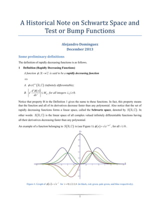
![Of course, any complex valued infinitely differentiable function having a compact support [i.e.,
C0 ,
] belongs to S
a maximum in
,
. This is so since any derivative of
is continuous and x i j x has
. Particularly, these last functions are called test functions or bump functions. The
linear space of test functions is denoted as D ,
. Of course this last space is a subspace of S
,
.
A function of this type is (see Figure 2).
1 2
1 x
x e ,
0,
x 1;
x 1.
Figure 2. Example of a test or bump function.
This is probably one of the simplest examples of a test function; however, it has an awful property. In fact,
following an argument similar to that given on p. 16 of (Griffel, 2002), since support of is the interval
1,1 , then x 0
about
for x 1 and x 1 , so all derivatives vanish at 1 . Hence the Taylor series of
1 is identically zero. But x 0 for 1 x 1 , so does not equal its Taylor series. Test
functions are thus peculiar functions; they are smooth, yet Taylor expansions are not valid. The above
example clearly shows singular behavior at x 1 .
Notice that in the theory of distributions, it is not necessary to use explicit formulas for rapidly decreasing
functions or test functions: They are used for theoretical purposes only.
Another related set of functions are the so-called functions of slow growth.
2
Definition (Functions of Slow Growth)
f:
is said to be a function of slow growth
A.
f C ,
;
B. There exists a B 0 such that
d j f x
dx
j
as
O x
2
B
x .](data:image/gif;base64,R0lGODlhAQABAIAAAAAAAP///yH5BAEAAAAALAAAAAABAAEAAAIBRAA7)
Empfohlen
Empfohlen
Weitere ähnliche Inhalte
Was ist angesagt?
Was ist angesagt? (20)
Andere mochten auch
Andere mochten auch (20)
Ähnlich wie A historical note on schwartz space and test or bump functions
Ähnlich wie A historical note on schwartz space and test or bump functions (20)
Mehr von Alejandro Domínguez Torres
Mehr von Alejandro Domínguez Torres (20)
Kürzlich hochgeladen
Kürzlich hochgeladen (20)
A historical note on schwartz space and test or bump functions
- 1. A Historical Note on Schwartz Space and Test or Bump Functions Alejandro Domínguez December 2013 Some preliminary definitions The definition of rapidly decreasing functions is as follows. 1 Definition (Rapidly Decreasing Functions) A function : is said to be a rapidly decreasing function A. C , B. xi d j x dx j (infinitely differentiable); M ij , for all integers i, j 0 . Notice that property B in the Definition 1 gives the name to these functions. In fact, this property means that the function and all of its derivatives decrease faster than any polynomial. Also notice that the set of rapidly decreasing functions forms a linear space, called the Schwartz space, denoted by S , other words: S , . In is the linear space of all complex valued infinitely differentiable functions having all their derivatives decreasing faster than any polynomial. An example of a function belonging to S , Figure 1. Graph of x x e i x 2 is (see Figure 1) x xi e x 2 , for all i 0 . for i 0,1, 2, 3, 4 (in black, red, green, pale green, and blue respectively). 1
- 2. Of course, any complex valued infinitely differentiable function having a compact support [i.e., C0 , ] belongs to S a maximum in , . This is so since any derivative of is continuous and x i j x has . Particularly, these last functions are called test functions or bump functions. The linear space of test functions is denoted as D , . Of course this last space is a subspace of S , . A function of this type is (see Figure 2). 1 2 1 x x e , 0, x 1; x 1. Figure 2. Example of a test or bump function. This is probably one of the simplest examples of a test function; however, it has an awful property. In fact, following an argument similar to that given on p. 16 of (Griffel, 2002), since support of is the interval 1,1 , then x 0 about for x 1 and x 1 , so all derivatives vanish at 1 . Hence the Taylor series of 1 is identically zero. But x 0 for 1 x 1 , so does not equal its Taylor series. Test functions are thus peculiar functions; they are smooth, yet Taylor expansions are not valid. The above example clearly shows singular behavior at x 1 . Notice that in the theory of distributions, it is not necessary to use explicit formulas for rapidly decreasing functions or test functions: They are used for theoretical purposes only. Another related set of functions are the so-called functions of slow growth. 2 Definition (Functions of Slow Growth) f: is said to be a function of slow growth A. f C , ; B. There exists a B 0 such that d j f x dx j as O x 2 B x .
- 3. The set of functions of slow growth is denoted as N , polynomial is an element of N , . Moreover, if . From this definition it is obvious that any f N , and S , , then f S , . It should also be observed that (Lighthill, 1958, p. 15) calls the elements of S , while the elements of N , good functions, fairly good functions. The historical note The Schwartz space is called so after the French mathematician Laurent Moise Schwartz (March 5, 1915 – July 4, 2002). This space was actually defined by Schwartz in his paper (Schwartz, 1947-1948). In fact, on p. 10 of this paper it can be read the definition of the Schwartz apace and its relation to the space of test functions: Main Scientists on Schwartz Space and Test or Bump Functions Soit S l’espace des fonctions x1 , x2 , xn indéfiniment dérivables (au sens usuel), et tendant vers 0 à l’infini plus vite que 2 2 toute puissance de 1 r ( r 2 x12 x2 xn ) ainsi que chacune de leurs dérivées. On peut encore dire que, si S , tout produit d’un polynôme par une dérivée de (ou toute dérivée du produit de par un polynôme) est une fonction bornée, et réciproquement ; nous dirons pour abréger que est «à décroissance rapide à l’ ainsi que ses dérivées». L’espace S admet évidemment, comme sous-espace particulier, l’espace D , des fonctions indéfiniment dérivables à support compact. Nous introduirons dans S Portrait 1. Laurent Moise Schwartz (March 5, 1915 – July 4, 2002) (http://wwwhistory.mcs.standrews.ac.uk/Biographies/ Schwartz.html). une notion de convergence. Des j S convergeront vers o si le produit par tout polynôme de toute dérivées des j (ou toute dérivée du produit des j par tout polynôme) converge uniformément vers o dans tout l’espace. On voit que des j D , convergeant vers o dans D , convergent aussi vers o dans S , mais la réciproque est inexacte. On montre aisément que D , considéré comme sous-espace vectoriel de S , avec la topologie induite par celle de S , est dense dans S . The method of multiplication of a suitable function by a test function and then integrate the result (as it is the case of the Theory of Distributions) is as old as the beginning of mathematical analysis. On years 1759-1760, the Italian born mathematician Joseph-Louis Lagrange (January 26, 1736 – April 10, 1813) published a paper where this method is used in relation to the integration of the sound wave equation (Lagrange, 1759-1760). On §6 Lagrange established the next problem and a method for finding its solutions: 6. Problème I. Étant donné un système d’un nombre infini de points mobiles, dont chacun dans l’état d’équilibre soit déterminé 3 Portrait 2. Joseph-Louis Lagrange (January 26, 1736 – April 10, 1813) (http://www-history.mcs.standrews.ac.uk/Biographies/ Lagrange.html).
- 4. par la variable x , et dont le premier et le dernier, qui répondent á x 0 et à x a soient supposés fixes, trouver les mouvements de tous les points intermédiaires, dont la loi est contenue dans la d2z d 2z formule 2 c 2 , z étant l’espace décrit par chacun d’eux dt dx durant un temps quelconque t . Qu’on multiplie cette équation par Mdx , M étant une fonction quelconque de x , et qu’on l’intègre en ne faisant varier que x ; il est clair que si dans cette intégrale, prise en sorte qu’elle évanouisse lorsque x 0 , on fait x a , on aura la somme de toutes les valeurs particulières de la formule d2z d 2z Mdx c 2 Mdx , qui répondent à chaque point mobile du 2 dt dx système donné. Cette somme sera donc Portrait 3. Norbert Wiener (November 26, 1894 – March 18, 1964) (http://www-history.mcs.standrews.ac.uk/Biographies/ Wiener_Norbert.html). d 2z d 2z Mdx c 2 Mdx . dt 2 dx This method was also used by Norbert Wiener on 1926 for solving linear partial differential equations of second order (Wiener, 1926). On pp. 582 Wiener wrote: 8. Operational Solution of Partial Differential Equations. Before we enter in this topic in detail, it is important to consider the nature of the solution of a partial differential equation. Let us consider the linear equation A 2u 2u 2u u u B C 2 D E Fu 0 , x 2 xy y x y Portrait 4. Kurt Otto Friedrichs (September 28, 1901 – December 31, 1982) (http://www-history.mcs.standrews.ac.uk/Biographies/ Friedrichs.html). where for simplicity’s sake, we shall suppose that the coefficients have as many derivatives as we shall need in the work which follows. If u satisfies this equation, it must manifestly possess the various derivatives indicated in the equation. As is familiar, however, in the case of the equation of the vibrating string, there are cases where u must be regarded as a solution of our differential equation in a general sense without possessing all the orders of derivatives indicated in the equation, and indeed without being differentiable at all. It is a matter of some interest, therefore, to render precise the manner in which a nondifferentiable function may satisfy in a generalized sense a differential equation. Let G x, y be a function positive and infinitely differentiable within a certain bounded polygonal region R on the XY plane, vanishing with its derivatives of all orders on the periphery of R . Then there is a function G1 x, y such that 4 Portrait 5. Jean Leray (November 7, 1906 – November 10, 1998) (http://www-history.mcs.standrews.ac.uk/Biographies/ Leray.html).
- 5. Au xx Bu xy Cu yy Du x Eu y Fu G x, y dxdy R u x, y G1 x, y dxdy R for all u with bounded summable derivatives of the first two orders, as we may show by integration by parts. Thus the necessary and sufficient condition for u to satisfy our differential equation almost everywhere is that u x, y G x, y dxdy 0 1 R For every possible G (as the G s for a complete set over any region), and that u possesses the requisite derivatives. Portrait 6. Sergei Lvovich Sobolev (October 6, 1908 – January 3, 1989) (http://www-history.mcs.standrews.ac.uk/Biographies/ Sobolev.html). Other famous mathematicians have also used the method of multiplication of a suitable function by a test function and then integrate the result; e.g., (Leray, 1934), (Sobolev, 1936), (Courant & Hilbert, 1937), (Friedrichs, 1939), (Weyl, 1940), (Schwartz, 1945), (Bochner & Martin, 1948). The test or bump functions D , properties have an interesting history: holding the following two additional x dx 1 ; lim x; lim 0 1 x x 0 n Until the year 1944 these functions does not have a specific name. It was in this year when, in the study of differential operators, the German born and American mathematician Kurt Otto Friedrichs (September 28, 1901 – December 31, 1982) proposed the name “mollifier” (Friedrichs, 1944, pp. 136139). Portrait 7. Richard Courant (January 8, 1888 – January 27, 1972) (http://wwwhistory.mcs.standrews.ac.uk/Biographies/ Courant.html). According to Wikipedia in its entry “Mollifier”, the paper by Friedrichs (http://en.wikipedia.org/wiki/Mollifier - cite_note-Laxref-0) […] is a watershed in the modern theory of partial differential equations. The name of the concept had a curious genesis: at that time Friedrichs was a colleague of the mathematician Donald Alexander Flanders, and since he liked to consult colleagues about English usage, he asked Flanders how to name the smoothing operator he was about to introduce. Flanders was a puritan so his friends nicknamed him Moll after Moll Flanders in recognition of his moral qualities, and he suggested to call the new mathematical concept a “mollifier” as a pun incorporating both Flanders’ nickname and the verb ‘to mollify’, meaning ‘to smooth over’ in a figurative sense. [The Soviet mathematician ] Sergei [Lvovich] Sobolev [October 6, 1908 – January 3, 1989] had previously used mollifiers in his epoch making 1938 paper containing the proof of the Sobolev 5 Portrait 8. David Hilbert (January 23, 1862 – February 14, 1943) (http://www-history.mcs.standrews.ac.uk/Biographies/ Hilbert.html).
- 6. embedding theorem [Sobolev, S. L. (1938). Sur un théorème d’analyse fonctionnelle. (in Russian, with French abstract), Recueil Mathématique (Matematicheskii Sbornik), 4(46)(3), 471– 497], as Friedrichs himself later acknowledged [Friedrichs, K. O. (1953). On the differentiability of the solutions of linear elliptic differential equations. Communications on Pure and Applied Mathematics VI (3), 299–326]. There is a little misunderstanding in the concept of mollifier: Friedrichs defined as “mollifier” the integral operator whose kernel is one of the functions nowadays called mollifiers. However, since the properties of an integral operator are completely determined by its kernel, the name mollifier was inherited by the kernel itself as a result of common usage. Portrait 9. Hermann Klaus Hugo Weyl (November 9, 1885 – December 9, 1955) (http://www-history.mcs.standrews.ac.uk/Biographies/ Weyl.html). Portrait 10. Salomon Bochner (August 20, 1899 – May 2, 1982) (http://wwwhistory.mcs.standrews.ac.uk/Biographies/ Bochner.html). References Bochner, S. & Martin, W. T. (1948). Several complex variables. Princeton, USA: Princeton University Press Courant R. & Hilbert, D. (1937). Methoden der Mathematischen Physik, II. Berlin, Deutschland: Verlag von Julius Springer (see pp. 469-470). Griffel, D. H. (2002). Applied functional analysis. New York, USA: Dover. Friedrichs, K. O. (1939). On differential operators in Hilbert spaces. American Journal of Mathematics, 61, 523-544. Friedrichs, K. O. (1944). The identity of weak and strong extensions of differential operators. Transactions of the American Mathematical Society, 55, 132–151. Lagrange, J. L. (1759-1760). Nouvelles recherches sur la nature et la propagation du son. Miscellanea Taurinensia, II (Œuvres de Lagrange, Tome Premier (1867), 150-316, Gauthier-Villars, France: Paris. 6
- 7. Leray, J. (1934). Sur le mouvement d’un liquide visqueux emplissant l’espace. Acta Mathematica, 61, 193-248. Lighthill, M. J. (1958). Introduction to Fourier analysis and generalised functions. Cambridge, United Kingdom: Cambridge University Press. Schwartz, L. (1945). Généralisation de la notion de fonction, de dérivation, de transformation de Fourier, et applications mathématiques et physiques. Annales de l’université de Grenoble, 21, 57-74. Schwartz, L. M. (1947-1948). Théorie des distributions et transformation de Fourier. Annales de l’université e Grenoble, 23, 7-24. Sobolev, S. L. (1936). Méthode nouvelle à résoudre le problème de Cauchy pour les équations linéaires hyperboliques normales. Matematicheskiui Sbornik, 1 (43), 39-71 Weyl, H. (1940). The method of orthogonal projection in potential theory. Duke Mathematical Journal, 7, 411-444. Wiener, N. (1926). The operational calculus. Mathematische Annalen, 95, 557-584. 7