Critical Evaluation Of The Success Of Monetary Policies
1. CRITICAL EVALUATION OF THE SUCCESS OF MONETARY POLICIES AGAINST
INFLATION IN TURKEY AFTER 1980
ABSTRACT
The most commonly known view on the relationship between money supply and inflation in
contemporary literature which is called as Monetarists’ view is that the increase in money supply
in the short-run may affect the real sector but in the long run will affect only the price level.
According to this point of view, monetary policy implementations in Turkey have been analyzed
year by year, and the effects of the monetary policy tools against inflation have been analyzed
and evaluated. Granger’s Causality Analysis is applied to determine cause-effect relation
between the CPI (dependent variable) and the independent variables, M2 money supply, RRR
(Required Reserve Ratio) and DR (Discount Rate) consecutively. According to the results of the
study, there is bilateral causality between money supply (M2) and the inflation level as it is
determined by the Granger’s Causality Analysis. M2 and RRR affect inflation rate after around
one-year period and DR affects inflation rate after circa four years period. In fact, the theory also
suggests that among the monetary policy tools, Discount Rate exerts its effect later than the other
tools. In Turkish economy, current inflation rate is the result of accumulation of past
experiences. Namely, current inflation rate is determined by recent cost and demand dynamics
along with the expectations of agents with a time lag. One of the major findings of this study is
that the increase in inflation rate actually leads to increase in money demand that leads to
increase in M2 money supply, which is the source of further price increases in Turkish economy.
If these factors determining the current inflation rate persist in the future, there is no doubt that
the future inflation will be no different from the present and the past.
Keywords: Monetary Policy, Inflation, Granger-Causality Analysis
JEL Classifications: E52
2. 1. Introduction
Every individual seeks for equilibrium and stabilization in his/her life. Like everyone, nations
also seek for equilibrium and stabilization. Economic stabilization is an important element for
the welfare of society. There is need to know the fundamental roles of the macro variables of the
economy, so that with proper economic policies stabilization can be achieved. According to
Monetarism, the main reason for business cycles in an economy is the cycles in the money
supply. These business cycles create instability and problems in the economy, which monetary
policy has a very important role in achieving stability (Flemming, 1978).
According to Monetarism, the main reason of economic instability is the up and down floats
of the money. Instability of the increase in money supply causes instability in the aggregate
demand. To get the stability in the aggregate demand and hence stability in growth, money
supply should increase at a stable rate (Ghosh and Phillips, 1998).
If the stabilization in the economy could not be reached, there will be several problems like
inflation, trade deficits, balance of payment problems, etc (Nessén, 2002). However, the most
important problem will be the negative psychological outcomes of these undesirable situations
(Flemming, 1978).
There are several studies related to this topic in the literature. Some of them are: According to
Kadioglu at al. (Kadioglu et al., 2000) macroeconomic policies have many goals like low
inflation, high economic growth, balance of payment equilibrium, etc. Since the monetary policy
has more flexible framework and exerts its effect with long and variable lags, it has certain
advantages over fiscal policy. The issue with the monetary policy is that as it is widely accepted
today, the central banks can only control inflation rates in the long run (Kuttner and Posen,
1999). In 1990s after the failure of monetary and nominal exchange rate targeting to reduce
inflation rates, Inflation Targeting (IT) is implemented successfully in some developed countries,
which encouraged developing and transition countries fighting against the high inflation rates.
2
3. Leading indicator approach is applied to a group variable theoretically defined to be potential
factors of inflation. Hodrick-Prescott, Beveridge-Nelson and band-pass methods are utilized and
the results are discussed. Empirical results of the analysis show that leading indicators of price
cycle and inflation can be achieved. Long-term, strongly inflation correlated indicators are
mostly identified by the band-pass filter. The common set of leading indicators derived using
suggested detrending methods increases reliability of the results. Using the without weighting
cross-correlation coefficient weighting and factor loading weighting of principal component
analysis, composite leading indices are constructed from the leading indicators. Granger-
Causality test is used to investigate the contribution of composite leading indicators to the
prediction of price cycle and inflation. The results indicate that composite leading indices may
help to predict price cycle and inflation (Ugur, 1999).
Relationships among inflation rate, exchange rate, money growth and budget deficits in
Turkey are also analysed using 1987:1-1997:4 quarterly data employing Johansen`s co
integration procedure. In the study two significant co integration relations are identified. The first
estimate co integration vector is the nominal money supply growth function, which is positively
affected from inflation rate and the budget deficits, and negatively affected from exchange rate
depreciation. The second significant co integration relation is interpreted as the inflation
equation. In this equation money growth, budget deficits and exchange rate depreciation
positively affect inflation rate, even though money growth, exchange rate depreciation are also
inflationary, the budget deficit is estimated as the most effective factor behind high inflation
(Saygili, 1998).
Yetman (Yetman, 2005) tries to demonstrate the sensitivity of price level targeting which is
proposed as an alternative to inflation targeting that may confer benefits if a central bank sets
policy under discretion, even if society’s loss function is specified in terms of inflation volatility.
Moreover, Shirvani and Wilbratte (Shirvani and Wilbratte, 1994) finds that money and inflation
are related only in countries with high inflation like Turkey.
3
4. On the other hand, Inflation is not only a monetary phenomenon but also has an expectational
character. By employing quarterly data for the Turkish Economy from the first quarter 1980 until
the last quarter of 1992, a set of stable long run relationships between various economic
variables that have a predictive power future movement regarding some major macroeconomic
movements in Turkey is obtained. Annual and seasonal unit root properties of the series are
investigated. We observed a close relation between increases in credits, international reserves
and aggregate demand that forms a loop which creates inflation (Izmirli, 1994).
Berumenta and Froyen (Berumenta and Froyen, 2006) assesses the effect of federal funds rate
innovations on longer-term nominal interest rates across different periods. Their evidences
suggest that these responses change with changes in the monetary policy regime.
In this study, it is aimed to determine extent, proximity in time and direction of the cause and
effect relation between monetary policy tools and high and persistent inflation rate in Turkish
economy. Therefore, indicator of inflation is taken as changes in CPI. Apart from the two
monetary policy tools Discount Rate (DR) and Required Reserve Ratio (RRR), as the indicator
of third monetary policy tool, which is Open Market Operations (OMO), M2 (M1, demand
deposits and time deposits) is taken. Required Reserve Ratio (RRR) and M2 money supply have
faster effects on inflation rate while Discount Rate (DR) has a longer period to this effect as is
pointed out by the theory. According to the literature survey conducted, the various studies on
related topics have mostly investigated only correlation (R2) between the inflation rate and the
related independent variables. However, not being content with just a correlation, in this study a
cause and effect relation is investigated between CPI and abovementioned independent variables.
To this aim, Granger- Causality Analysis is used.
Inflation is perhaps the most significant economic problem facing Turkey and its origin
mainly lies in imbalances and improperly used monetary policies. The main motivation behind
this paper is to explore some of the key reasons of Turkish inflation and the relationship between
the inflation rate and the monetary policy tools applied in the economy since 1980. In this frame,
4
5. in the second section of the study an overview of monetary sector in Turkish economy for the
analysed period is given. In the following section Granger-Causality Analysis is presented and
applied. Findings that are obtained by the analysis are evaluated in the fourth section. Finally,
study ends with conclusion which provides some recommendations.
2. An Overview of the Developments in Monetary Sector in Turkish Economy After 1980
Inflation is chronic and very high in Turkey since late 1970s. There are several reasons, which
increase the inflation rate, and also several outcomes of the high inflation, one of which is the
general psychology of the citizens of Turkey having expectations in the direction of increase in
inflation (Kesriyeli, 1997).
Since economy affects all the aspects of individual lives, inflation creates an unstable life
structure such as decrease in purchasing power of the money, lower life standards especially for
the people who earn fixed income. Also inflation creates a deeper difference in social standards
among the citizens (Flemming, 1978).
“Inflation expectation is one of the main reasons of the increasing inflation observed in
Turkish economy. In a chronic inflationary environment, agents respond more rapidly to the
available information in the market.” (Kandiller, 1997). What are the deeper reasons and the
phases of inflation in Turkey that caused it to have a chronic nature? In fact, along with the effect
of expectations, it has been disclosed in the recent, April 2002 money report of the Central Bank
that an increase in price level is the cause of 2002 money report of the Central Bank that an
increase in price level is the cause of increased demand for money in the economy, which
necessitates an increase in M2 money supply. This increase in money supply in turn leads to
increase in price level (CBRT, 2002). This vicious circle effect is in fact found out in the results
of the Granger-Causality Analysis utilized in this study. This perpetual interaction between the
money supply and price level may be the basis of the abovementioned chronic nature of inflation
in Turkey.
5
6. Turkey has undergone a staged liberalization over quite a long period. The 1980 liberalization
represents a more fundamental attempt by the government to commit to a more open trade
regime and a liberalized financial system. There were several objectives: stabilization of the
balance of payments, rationalization of the foreign exchange system, improved efficiency of
state enterprises, a boost to the private sector and encouragement of worker remittances and
foreign direct investment (Tukel, 1986).
However, along with the abovementioned liberalization efforts, at least to control the ensuing
inflation, monetary policies have gained an important role in the economy. Since the control of
inflation can be achieved through the control of money stock in the economy, especially
monetary policies in a contractionary nature were applied. Independence of the Central Bank
from the Treasury was a key priority for Turkey to set proper monetary policies (Ertugrul and
Selcuk, 2000). Despite substantive reforms and sophistication in the conduct of monetary and
exchange rate policies, inflation has never been the ultimate policy goal of the monetary
authorities in Turkey for a long time.
As can be observed from the five-year background additional statistical data before 1980, the
sudden three-digit inflation rate of 1980 can be attributed to circa 80% increase in the increase
rate of M2 in 1979. This finding reinforces the results of Granger-Causality Analysis, which
gives a mutual casual relation between M2 and inflation with around 1 and 2-year lags
consecutively. That is, the increase in CPI, from 16% in 1976 to 22.5% in 1977, caused an
increase in M2 after around 2-year lag from 34.4% in 1978 to 61% in 1979. And in turn, the
increase in M2 in 1979, almost doubling it compared to 1978, has caused an increase in inflation
rate of 1980 which is also almost double of the previous year.
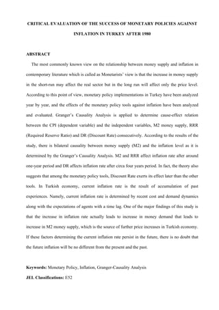
Table 1. Inflation rate, M2 money supply, Discount Rate (DR), Required Reserve Ratio (RRR)
Years Inflation Rate M2 (Billion M2 (% DR RRR
(%) TL) Change) (%) (%)
1975 19 147 30 9 20
6
8. 1994 60.81 155.66 17.43 6.67
1995 -17.21 -19.33 -10.93 12.5
1996 -8.63 33.61 0 -11.11
1997 6.71 -29.59 31.57 0
1998 -1.39 8.98 0 0
1999 -23.28 -9.16 13.33 -25
2000 -39.9 -51.15 -7.69 0
As for the effect of DR on CPI, the increase of DR from 10.25% in 1979 to 26% in 1980 gave
its inverse effect on inflation rate 4 years later, decreasing it from 107.2% in 1980 to 48.4% in
1984, as has been econometrically determined by Granger-Causality Analysis. Also the inverse
effect of increase in RRR, from 19% in 1979 to 30% in 1980, on inflation rate can be seen in
1981 after around 1-year lag, such that inflation rate was 107.2% in 1980 and it decreased to
36.8% in 1981.
In this part, the analysis of the effects of monetary policy tools (DR, RRR, M2) on inflation
rate having their lags as mentioned above for the first eight years of the observation period of
this study is explained. M2 money supply is taken as one of the independent variables (DR,
RRR, M2) and inflation rate is taken as dependent variable in the econometric section of this
study.
Turkey has been burdened by high inflation actually since late 1970s. In recent years, this
problem became more chronic as inflation rates have steadily increased. Past economic
stabilization programmes designed to fight with inflation have never been successfully carried
through. Besides expansionary fiscal and monetary policies, low interest rates and wrong
exchange rate policies have caused to increase the instability of the economy (Barutca, 2000).
“During 1978-1979 Turkish economy had been in a deepening crisis with inflation and balance
of payment difficulties. Immediately after that, the government announced a major stabilization
programme on 24th January 1980, which included a series of new economic measures that were
intended to solve the hyper-inflation, economic stagnation and unmanageable balance of
payment deficits.” (Alper and Ucer, 1998).
8
9. As is known from the theory, monetary policy has its effects on the economy in a relatively
shorter period compared to fiscal policy. Accordingly, monetary policy tools in Turkish
economy have been used for short-term stabilization. These tools affected the inflation rate in
around 1 to 4-year periods. Since in our econometric model of Granger-Causality Analysis AIC
and SIC gave 1 to 4-year lags as optima, in the Tables 3.1 and 3.2 the values from 1975 onwards
are included as background information to have a healthy analysis of the two decades from 1980
to 2000.
With the economic package of 24th January 1980; government started implementing tight
monetary policy. However, inflation rate in this year was as high as 107.2%. Discount Rate (DR)
was increased to 31.5% in 1981 with an increase of 21.15% compared to 1980. However
Required Reserve Ratio (RRR) was kept at the same level (30%) in 1980. According to the
results achieved in Granger Causality Analysis, DR would affect inflation rate after circa 4 years
period. Actually it happened in this way, inflation rate decreased by 58% from 107.2% in 1980
to 45% in 1985. The increase in M2 money supply was 84.95% in 1981 and it started to decline
after this year until 1984. As the Granger-Causality Analysis shows, M2 money supply affects
inflation rate after around 1-year lag, and in turn, inflation rate affects M2 money supply
approximately after 2 years. In fact, the 5.5% increase in inflation rate, from 54% in 1978 to 57%
in 1979, has caused 13.26% increase in the increase of M2 in 1981 after 2 years, from 75% in
1980 to 84.95% in 1981, in turn, the increase in M2 led to increase in inflation rate after around
1 year, from 27% in 1982 to 31.4% in 1983. Similar cause and effect chain relations can be seen
between the years 1980-1987. Although little changes in the increase rate of M2 are observed in
some years between 1980-1987 periods, an absolute decrease in the increase rate of M2 money
supply is observed at the end of this period. Accordingly, inflation rate also decreases by 64%
from 107.2% to 38.6% between these years.
“The excess issue of money only produces price rises by the Central Bank, probably acting
under orders from the government. According to Monetarists, therefore, inflation can only be
9
10. brought under control by determined action by the government to restrict increases in the money
supply.” (Kuttner and Posen, 1999).
Required Reserve Ratio (RRR) other monetary policy tool was kept stable between the years
1980-1982. As is known from Chapter 4, RRR has an effect on inflation rate in around 1 year
period. Required Reserve Ratio was decreased by 16.66% from 30% to 25% in 1983. Its effect
was seen in 1984 after 1-year lag as an increase in inflation rate by 54.14% from 31.4% to
48.4%. RRR was kept stable at 25% until 1984. Although it was decreased by 24% to 19% in
1985, it did not affect inflation rate in an increasing way in 1986. In the year 1986, monetary
policy implementations had a turning point, Central Bank started to control the commercial
banks` reserves through Open Market Operations (OMO). “Starting Open Market Operations
(OMO) became the new way to help the control of quantity of money besides Required Reserve
Ratio and Discount Rate” (Kesriyeli, 1997).
Other effects of RRR on inflation rate were seen in 1987 and 1988 such as; it was decreased
to 15% in 1986 and inflation rate increased to 38.6% in 1987; it was decreased to 14% in 1987
and was kept at that level until 1988, inflation rate increased to 73.7% in 1988.
“There was persistent increase of inflation at around the time of the 1988 stabilization efforts,
which indicates perhaps public’s loss of confidence in the battle against inflation in the face of
deteriorating fiscal balances.” (Alper and Ucer, 1998). Central Bank liabilities became more
liquid and more controllable. Central Bank became more elastic in applying the monetary policy.
“The base of the credit policy of the Central Bank was to support the production and export of
manufacture and agricultural sectors. So, until the end of the year, Central Bank credits were
used to finance the growing sectors rather than to use it as a tool of monetary policy. Hence,
Discount Rates were regulated to be a new monetary policy tool instead of being selective credit
policy tool.” (Barutca, 2000). Since the credits were given to support the abovementioned
sectors, the increase in M2 money supply, 54.1% in 1988, has not been inflationary in 1989.
10
11. Discount Rate was increased by 20% to 54% in 1988; therefore, disinflation effect was seen
in 1992. Inflation rate in 1992 decreased to 70.1%. M2 money supply was increased by 35.58%
to 73.34% in 1989, however, it did not affect inflation rate in an increasing way in 1990.
Required Reserve Ratio (RRR) was decreased to 10% in 1989. The expected effect of decrease
in RRR is increase in inflation rate but actually in 1990 a little decrease in inflation rate is
observed. This unexpected decrease of inflation may be explained by increase in the confidence
level of the public after the start of implementation of the aforementioned stabilization efforts.
“1990 became another turning point in the history of the Turkish economy such that, in this
year Central Bank started to declare its monetary programme to the public (transparency of the
Central Bank operations) for the first time. Monetary policies in 1990-1991 were in agreement
with the rules for the economic stabilization offered by the Monetarists (rule-based policies).”
(Kandiller, 1997). “But soon monetary policies were changed and policies were started to be
implemented according to the equilibrium in different markets in the economy” (Kesriyeli,
1997). For instance, inflation rate increased by 90.93%, from 38.6% in 1987 to 73.7% in 1988,
and it led to an increase in the increase of M2 by 22.79%, from 51.82% in 1990 to 63.63% in
1991, and in turn, it has caused an increase in inflation rate to 70.1% in 1992. The 4.73%
decrease in inflation rate in 1990 has caused 1.19% decrease in the increase rate of M2 in 1992.
It affected inflation rate after 1 year. Actually, inflation rate decreased from 70.1% in 1992 to
66.1% in 1993.
Until 1994, monetary targets had been mostly achieved by following the new programme, and
accordingly stabilization target at the money markets was achieved to a great extend by a
decrease in inflation rate as mentioned above. “The Gulf War that started in 1991 and some other
political events and early elections made the monetary policy inapplicable. Besides, crisis
affected oil prices very badly, oil prices increased very fast and hence, production costs
increased also. Increase in production costs caused an increase in the overall price level, which
caused also an increase in the inflation rate. This led to depreciation of TL. Economy came to a
11
12. crisis, high and continuous inflation rate led to increase in real exchange rate constituted one of
the reasons of January 1994 crisis.” (Barutca, 2000).
On 5th April 1994, the economic package was declared. This economic package was geared
to achieve a fast decrease in inflation rate to achieve stabilization in fiscal sector and exchange
rates (Alper and Ucer, 1998). Discount Rate and Required Reserve Ratio was increased to
achieve the stabilization in the economy. In fact, Discount Rate was increased by 17.43%, from
54.5% in 1993 to 64% in 1994, and Required Reserve Ratio was increased by 6.67%, from 7.5%
in 1993 to 8% in 1994.
Discount Rate has its full effect on inflation rate around 4 years lag. Thus, the full effect of
increase in Discount Rate in 1994 can be seen in the year 1998. Inflation rate decreased to 84.6%
in that year. Together with this, Required Reserve Ratio was increased to 8% in 1994. Its full
effect on inflation rate was seen after 1-year lag in 1995, in that year inflation rate decreased to
88%. At the following year, RRR was increased again to the 9% level. It has affected inflation
rate in 1996, inflation rate decreased to 80.4% in that year.
M2 money supply was regulated to achieve disinflation efforts of 5th April 1994 economic
package. The increase rate of M2 decreased to 99.36% in 1995 as a result of 5.7% decrease in
inflation rate, from 70.1% in 1992 to 66.1% in 1993. The decrease in the increase of M2 in 1995
has caused a decrease in inflation rate from 88% in 1995 to 80.4% after 1 year in 1996.
n the middle of 1998, both Turkish economy and world economy went into a recession. The
main reason for the recession in Turkey was decrease in domestic demand (Barutca, 2000). “The
main functions of the money demand are, growth rate, inflation and interest rates. But this is not
the usual case especially if we consider the Turkish economy. The quantity of money that people
want to have does not depend mostly on the inflation rate.” (Kesriyeli and Kocaker, 1999).
Although an increase in M2 money supply is observed in 1998 (101.87%), inflation rate
decreased to 64.9% by the end of 1999.
12
13. In the year 1999, Central Bank declared its direct inflationary policy to the public. The
increase in M2 money supply was decreased to 92.53% in 1999 from 101.87% in 1998 and its
disinflationary effect can be seen 1 year later, inflation rate decreased from 64.9% in 1999 to
39% in 2000. Discount Rate was increased from 57% in 1996 to 75% in 1997. This increase in
DR has caused a decrease in inflation rate by 39.9%, from 64.9% in 1999 to 39% in 2000.
The government on 9th December 1999, declared the 3-year disinflation programme. The
fundamental goals of the programme were; to bring down the consumer price inflation to 25% by
the end of 2000, 12% by the end of 2001 and 7% by the end of 2002. “Through the monetary
policy implemented in 1999, the Central Bank aimed at ensuring stability in financial markets.
Headline inflation may not represent long-term price movements. Short-term transitory changes
in inflation are generally the results of supply shocks. Non-monetary events such as, changing
seasonal patterns, seasonal shocks and sector specific shocks may cause transitory noise in short-
term price changes and may misrepresent long-term price movements.” (CBRT, 2002).
The main determinant of the developments in the Turkish economy in 2000 was the
“Disinflation Programme” which had been applied since the beginning of the year (CBRT,
2002). “At the beginning of the programme, the Required Reserve Ratio for Turkish Lira
denominated deposits were reduced from 8% to 6% where the remaining 2% was to be held as
free deposits at the Central Bank and subject to the public sector and realized the quarterly net
domestic assets targets, which were set as performance criteria in the programme.” (Ercel, 2000).
In the year 2000, monetary policy was similar to the 1999-stabilization programme. But a
financial crisis started on 22nd November 2000. Although the target rate of inflation was 25% by
the end of 2000, it realized as 39% at the end of that year.
3. The Granger-Causality Analysis Concerning the Interaction of Inflation and Basic
Monetary Policy Tools in Turkey
13
14. 3.1 “VAR” (Vector Autoregression) Lag Order Selections and “LM” (Lagrange Multiplier)
Test
The main objective of this study is to find out the nature of causality relationship between
monetary policy tools and inflation rate (D (CPI)) in Turkish economy. Those tools are taken as
Required Reserve Ratio (RRR), Discount Rate (DR) and M2 money supply, which are the main
monetary policy tools. Annual data starting from 1980 until 2000 are taken and the cause and
effect relations of changes in the abovementioned monetary policy tools (independent variables)
with the inflation rate (dependent variable). In Granger-Causality Analysis, there are four
possible outcomes regarding the cause-effect relation of basic monetary policy tools and
inflation rate in Turkey. “First, causality may run from the monetary policy tools to inflation rate
(CPI); second, it might run in the opposite direction; third, it may run in both directions
(implying the existence of feedback system); and fourth, they may turn out to be no evidence of
causality in either directions (Granger, 1969a).
“A Vector Autoregressive Model, or VAR for short, is a time series model used to forecast
values of two or more economic variables. Unlike simultaneous equations models, however, the
VAR model uses only past regularities and patterns in historical data as a basis for forecasting.
No structural model is built. Because no simultaneous equations model is needed, VAR models
provide a convenient basis for forecasting within sub regions of the country or at the state level.”
(Granger, 1969a). Suppose xt and yt are economic variables whose values we wish to forecast. A
VAR model for these variables is given by these equations:
yt = α0 + α1*yt-1 +………+ αp*yt-p + β1*xt-1 +…..+ βp*xt-p + εt
(1)
xt = α0 + α1*xt-1 +………+ αp*xt-p + β1*yt-1 +……+ βp*yt-p + ut
(2)
“In this model, the current value of a variable yt, is explained by lagged values of itself and
lagged values of the variable x, plus a random error et. Note that the current value of yt does not
14
15. depend directly on the current value xt, and thus, the two-equation model 1 and 2 is not a
simultaneous equations model. The random disturbance et, is assumed to have zero mean,
constant variance σe2, and to be serially uncorrelated. Similarly, the value of xt is explained by
its own lagged values, the lagged values of yt and the random disturbance ut. The random
disturbance ut is assumed to have mean zero, constant variance σu2, and to be serially
uncorrelated. Each of the variables xt and yt is explained by its lagged values, but no other
economic variables are involved. Thus the VAR model captures the historical patterns of each
variable and its relationship to the other.” (Granger, 1969a).
“The VAR model specified in equations 1 and 2 is called a two-dimensional vector
autoregressive model of order p; it is denoted by VAR (p). It is called two-dimensional because
it contains two variables and more equations; adding more variables and more equations can
increase its dimension. It is of order p because it contains lags up to order p. One problem of
model specification is selecting the length of lag. As for univariate time-series models and
distributed lag models, a variety of criteria are used, including the AIC and SIC criteria. No one
method has been found to be best, and there is a possibility of a misspecification when using any
method.” (Granger, 1969a).
Since most of the test procedures are based on regression analysis, it needs estimation to
ensure that the series satisfy the required stationary conditions. The Dickey-Fuller test is a more
formal test for the existence of a unit root (Henry and Shields, 2004). Applications of the
Dickey-Fuller and Augmented Dickey-Fuller unit-root tests to find the required stationary
condition show that (D (CPI) and M2 series are integrated at level 1 (I (1)). Hence, when
constructing a VAR (1) model relating to CPI and M2, we assumed that the I (1) nature of the
variables made it appropriate to set up a VAR model in first differences. RRR and DR series are
at I (0). Accordingly, particular emphasis is placed in all the statistical analysis henceforth.
(Augmented Dickey-Fuller Unit Root Tests on D (CPI), DR, RRR and M2 are shown in
Appendix B).
15
16. In this section the procedure and methodology of choosing the lag length is explained. “The
Lagrange Multiplier (LM) test begins with the null hypothesis which is given by the restricted
model (See equation 14). It asks whether a movement in the direction of the alternative
hypothesis can significantly improve the explanatory power of the restricted model. The LM test
is based on the technique of constrained maximization, in which a Lagrange multiplier is used to
provide an estimate of the extent to which the imposition of a constraint alters the maximum-
likelihood estimates of a set of parameters. Let βUR is the maximum-likelihood estimator of the
parameters of the unrestricted model and let βR represent the parameters associated with the
restricted model. Then our objective is to maximize ln L (βUR) subject to the restriction that
βUR=βR. This is equivalent to maximizing
ln L (βUR) - λ(βUR-βR) (3)
where λ is the Lagrange multiplier. The Lagrange multiplier measures the marginal
“valuation” associated with the constraint: the greater is λ, the greater is the reduction in the
maximum value of ln L (βUR) as the constraint becomes binding. To see this formally, note that
one of the first-order conditions for maximization is
∂ln(L)/∂βUR (4)
so that λ is the slope of the likelihood function. If the null hypothesis that the restrictions are
valid is not rejected, the restricted parameters will be close to the unrestricted parameters and the
value of λ will be small. The LM test, which is based on the magnitude of λ, sometimes is called
score test (LM= λ(βR`)2/I(βR`), where λ and I(), the information matrix, are calculated by
differentiation of the log-likelihood function.).
The Lagrange multiplier test can be easily applied to the special case in which one is
considering the possibility of adding additional explanatory variables to a regression model.
Suppose one has estimated the restricted model:
Y= β1 +β2X2 +…..+βk-qXk-q +εR (5)
16
17. and is considering the possibility of adding some or all of q additional variables that are
contained in the unrestricted model:
Y= β1 +β2X2 +…..+βk-qXk-q +……+βkXk +εUR (6)
The Lagrange multiplier test of the hypothesis that each of the additional q variables has a
coefficient of 0 is performed by first computing the residuals from the restricted model given by
Eq.(14). Specifically,
ε`R= Y-β1`-β2`X2-…-β`k-qXk-q (7)
Now consider the regression of these residuals on all the explanatory variables in the
unrestricted model:
ε`R= γ1+γ2X2+…+γkXk+u (8)
If all the additional variables were irrelevant, the coefficients would be zero on the k-q
variables that are added when we move from the restricted model to the unrestricted model.
The Lagrange multiplier test is determined on the basis of a test of significance of the
regression in Eq. (8). Specifically, the LM test statistic, which is given by LM=NR02 Follows a
chi-square distribution with q (the number of restrictions) degrees of freedom. N is the sample
size, and R02 is the R2 associated with the regression in Eq (8).” (Pindyck and Rubinfeld).
Choice of the correct lag length is essential while doing this LM test: In the choice of the
relevant lag length Akaike Information Criterion (AIC) and Schwartz Information Criterion
(SIC) are both informative. Therefore the abovementioned criterion tests are used for choosing
the optimum lag length to be taken in the Granger-Causality Analysis. In this study, the
observation period has been taken as 21 years (1980-2000). Relevant studies show that the
maximum lag length to be tested should be 4 with approximately 20 observations; since, it is
suggested for not to lose the important details of the information while testing the hypothesis.
Table 3. VAR order selection: Information criteria and LM (Lagrange Multiplier) test for serial
correlation.
17
18. LAG CPI DR RRR M2
AIC 1 0.230177 -0.462956 -0.811964 0.504675*
2 0.035425 -0.634415 * 0.605700
3 * -0.533639 -0.785934 0.722089
4 0.122790 -0.739242 -0.727775 0.853656
0.253434 * -0.605131
SIC 1 0.324584 -0.321346 -0.763677 0.551878*
2 0.177035 -0.445602 * 0.700107
3 * -0.297622 -0.689360 0.863699
4 0.311603 -0.456022 -0.582915 1.042470
0.489451 * -0.411983
LM-Stat 1 0.036978 0.052726 0.606131 0.218394
(SC (4)) 2 0.038471 0.670494 0.693090 0.279498
3 0.008677 1.200531 0.615239 1.907026
4 0.012100 0.687729 0.751161 1.821266
Probability 1 0.8475 0.8184 0.4362 0.6403
(msl) 2 0.8445 0.4129 0.4051 0.5970
3 0.9258 0.2732 0.4328 0.1673
4 0.9124 0.4069 0.3861 0.1772
SC (4): Serial Correlation with 4 lags, msl: Marginal Significance Level
*= The minimum value of the corresponding test (Shows the best lag length)
Minimum values of AIC and SIC give us the optimum lag length (“VAR” Lag Order
Selections and “LM” Test results are shown in Appendix D). Therefore, 4-lag for DR, 2-lag for
CPI, 1-lag for RRR and 1-lag for M2, which are shown in the above table giving the minimum
values for both tests, are selected as the optimum lag lengths and to be used in the causality
analysis. Since there is no serial correlation in any of the lags, the result achieved is
econometrically reliable.
18
19. The determinant (Ω) of the residual covariance is computed as (T: number of observations, it
is 21 in this analysis; ε: error term; p: the value which determines whether to reject or accept the
null-hypothesis by comparing it to the level of significance) (Granger, 1969: 426):
Ω= det { (1/ T-p)* ∑ε1*ε1′} (9)
The log likelihood value (L) is computed assuming a multivariate normal (Gaussian)
distribution as:
L = - T/2 {k* (1+log 2π)+log Ω} (10)
and the two information criteria are computed as:
AIC = -2L/T + 2n/T (11)
SIC = -2L/T + n log T/T (12)
n is the total number of estimated parameters in the VAR.
3.2 Granger’s Causality Analysis
The Granger (Granger, 1969b) approach to the question of whether X causes Y is to see how
much of the current Y can be explained by past values of Y and then to see whether adding
lagged values of X to them can improve the explanation. Y is said to be Granger-caused by X if
X helps in the prediction of Y, or equivalently if the coefficients on the lagged Xs are
statistically significant. Note that two-way causation is frequently the case; X Granger-causes Y
and Y Granger-causes X (Granger, 1969b).
“To evaluate whether each of these two conditions holds, we want to test the null hypothesis
that one variable does not help to predict the other. For example, to test the null hypothesis that
“X does not cause Y”, we regress Y against lagged values of Y and lagged values of X (the
unrestricted regression) and then regress Y only against lagged values of Y (the restricted
regression). A simple F-test can then be used to determine whether the lagged values of X
contribute significantly to the explanatory power of the first regression (F= (N-k) (ESSR-
ESSUR)/q (ESSUR), where ESSR and ESSUR are the sums of squared residuals in the restricted
19
20. and unrestricted regressions, respectively; N is the number of observations; k is the number of
estimated parameters in the unrestricted regression; q is the number of parameter restrictions.
This statistic is distributed as F (q, N-k)). If they do, we can reject the null hypothesis and
conclude that the data are consistent with X causing Y. The null hypothesis that “Y does not
cause X” is then tested in the same manner.
To test whether X causes Y, we thus proceed as follows. First, test the null hypothesis “ X
does not cause Y” by running two regressions:
Y= ΣmI=1 αI Yt-I + ΣmI=1 βI Xt-I +εt (Unrestricted regression) (13)
Y= ΣmI=1 αI Yt-I + εt (Restricted regression) (14)
And used the sum of squared residuals from each regression to calculate an F statistic and test
whether the group of coefficients β1,β2,……,βm are significantly different from zero. If they
are, we can reject the hypothesis that “X does not cause Y”. Second, test the null hypothesis “Y
does not cause X” by running the same regressions as above, but switching X and Y and testing
whether lagged values of Y are significantly different from zero.” (Pindyck and Rubinfeld).
In applying Granger’s test, the choice of lag length is usually seen as essentially arbitrary.
Since the best lag to be chosen 2 for D (CPI), 4 for DR, 1 for RRR, 1 for M2 according to the
both tests (AIC and SIC) in Granger’s Causality Analysis lag lengths are chosen as mentioned
before to have meaningful explanation in the abovementioned three monetary policy tools on the
inflation rate of Turkish economy.
The results, which are obtained when Granger’s test procedure is applied, are summarized in
the following tables. The results reported in the following tables are obtained with the optimum
lag lengths which are mentioned before according the results of the above AIC and SIC tests for
this study.
Degree of freedom k is 4 (There is 3 independent variables (DR, RRR, M2) including the
constant) and number of observations N is 21. For a test at a significance level of 0.05 where we
have 3 degrees of freedom (k-1) for the numerator and 17 degrees of freedom for the
20
21. denominator (N-4), the appropriate F value is found by looking under the 3 degrees of freedom
column and proceeding down to the 17 degrees of freedom row; there we find the appropriate
F3-17 (F critical) value to be 3.20. This F3-17 value is used in every causality analysis in this
test.
Table 4. Causality analysis between D(CPI) and DR
H01: DR does not Granger Cause D(CPI)
LAG 4
F-TEST 3.71517
PROBABILITY 0.07308
H02: D (CPI) does not Granger Cause DR
LAG 2
F-TEST 1.94584
PROBABILITY 0.18538
Table 5. Causality analysis between D (CPI) and RRR
H01: RRR does not Granger Cause D (CPI)
LAG 1
F-TEST 3.56867
PROBABILITY 0.08678
H02: D (CPI) does not Granger Cause RRR
LAG 2
F-TEST 1.93269
PROBABILITY 0.18723
Table 6. Causality analysis between D (CPI) and M2
H01: M2 does not Granger Cause D (CPI)
LAG 1
F-TEST 5.21007
PROBABILITY 0.03746
H02: D (CPI) does not Granger Cause M2
21
22. LAG 2
F-TEST 6.03676
PROBABILITY 0.01534
4. Evaluation of the Findings
The results reported in Table 4, show a unilateral causality from DR to D (CPI). 4th lag was
chosen for DR and 2nd lag was chosen for D (CPI) as they are determined by as the optimum
lags by AIC and SIC of the “VAR” Lag Order Selections and “LM” tests. The null-hypothesis
H01:’DR does not Granger Cause D (CPI)’ is rejected according to the F-test results at a 5%
significance level. To test for the possibility that causation also flows in the opposite direction
(thereby giving rise to feedback system) the reversed Granger test that is H02: ‘D (CPI) does not
Granger Cause DR’ is performed. The result of this test is such that the null-hypothesis is
accepted. Taken together, these results would seem to indicate during the two decades period in
question, DR causes D (CPI).
It can be suggested that there is a causality, which runs from the monetary policy tool (RRR)
to inflation rate D (CPI) and it can be seen in Table 5. The 1st lag was chosen for RRR and 2nd
lag was chosen for D (CPI) from the result of the VAR test. The first null-hypothesis H01: ‘RRR
does not Granger Cause D (CPI)’ is rejected according to the F-test result at a 5% significance
level. And the second null-hypothesis H02: ‘D (CPI) does not Granger Cause RRR ’ is accepted
means that D (CPI) does not cause RRR.
The results shown in Table 6 suggest the existence of feedback system. The 1st lag was
chosen for M2 and 2nd lag was chosen for D (CPI) as they are taken from the VAR test results
above. The null-hypothesis H01: ‘M2 does not Granger Cause D (CPI)’ and the second null-
hypothesis H02: ‘D (CPI) does not Granger Cause M2’ are both rejected at a 5% significance
level. Over the period in question, D (CPI) caused M2 while D (CPI) caused by M2.
Here Turkish data in an investigation of the relationship between the inflation rate D (CPI)
and monetary policy tools that are Discount Rate (DR), Required Reserve Ratio (RRR) and the
22
23. M2 money supply was used. The results were such that the relevant lags again were determined
by AIC and SIC tests as 4-lag for DR, 1-lag for RRR and 1-lag for M2 for their effects on D
(CPI). And as for D (CPI)`s effect on M2 the aforementioned criteria tests give 2-lag for D (CPI)
as optimum. Causality analysis of the Granger variety provides evidence of feedback system
between inflation rate (CPI) and M2 money supply. And there is a unidirectional causality
between Required Reserve Ratio (RRR) and inflation rate D (CPI) from RRR to D (CPI) and
between Discount Rate (DR) and inflation rate D (CPI) from DR to D (CPI).
5. Conclusion and Recommendations
In this study, monetary policy developments in Turkey have been analyzed year by year, and
the mutual effects of the monetary policy tools (DR, RRR, M2) and inflation (CPI) have been
econometrically tested with Granger-Causality Analysis. According to the results of the study,
during the observation period in Turkish economy, increase in inflation rate resulted in increases
in M2, and in turn, expansion in M2 gave rise to increase in the inflation rate. This has been one
of the major findings of this thesis, which has been verified by the econometric analysis
conducted by Central Bank of Turkey in April 2002. Also a unilateral causation of DR and RRR
on CPI with around 4 and 1-year lags consecutively has been found out.
Latest financial crises of November 2000 and February 2001 showed that it is very important
to implement serious monetary programmes because money supply regulations along with
interest and exchange rate policies play very important roles in the Turkish financial system.
Hence, they should be carefully regulated in order to have stable and low levels of inflation.
Thus, monetary policy gained importance after the abovementioned crises and the governments
tried to use the policies according to the Monetarist’s rules (i.e. rule-based policies).
Continuous inflation leads to expectations of persistent inflation for the future and as inflation
gets accelerated, it causes expectations of higher inflation rate for the coming years. This
becomes another problem while fighting with inflation. In Turkey especially after 1980,
23
24. monetary policies have been used to keep inflation at a stable level, but, never took direct
inflation targets; the importance of rule-based monetary policies have gained value but they were
applied auxiliary to fiscal policies. Fiscal and corresponding monetary policies in practice could
not reach the targets. Higher inflation expectations in Turkish economy were one of the main
causes of unsuccessful disinflation programs up to now.
According to Friedman’s “Money Demand Theory”, money supply should be targeted as
much as increase in money demand. In other words, for the monetary targeting to be successful,
monetary expansion should be consistent with the macroeconomic targets. There should not be
excess money supply. The following targets determine the main features of the last monetary
programme (CBRT, 2002):
a. Limiting the Net Domestic Assets of the banks, this is the operational target of the Central
Bank, throughout the new regulations brought to the banking sector.
b. Dispersion of excessive foreign borrowing obtained from IMF and World Bank, between
Central Bank reserves and consolidated budget financing.
However, these targets of the last monetary programme may further increase domestic debt, if
they are not applied appropriately.
For those who monitor the latest theoretical studies in economic literature and the country
experiences, it comes as no surprise that restoring economic fundamentals alone does not suffice
for reaching the abovementioned targets. Central Bank has important tasks for improving the
economic expectations. This relates to transparency, according to which a Central Bank should
announce the framework of prospective monetary policy, the changes in operational rules and
the rationale behind the decisions. Also the Economic and Social Council and the public sector,
due to pricing policy of the State Economic Enterprises have important obligations in getting rid
of backward indexation habits.
24
25. Actually along with the increase in the increase rate of money supply more than the required
level, the price setting based on past inflation (backward indexation), which as a result of
inflationary expectations is also one of the main reasons for inflation to be high in Turkey.
In short, the main causes of chronic inflation in Turkey could be summarized as; excessive
monetary expansion, inflation expectations and the accumulation of past experiences which is
determined by recent cost and demand dynamics along with the expectations of economic agents
with a time lag. If these factors determining the current inflation rate persist in the future, there is
no doubt that the future inflation will be no different from the present and the past. Actually, in
the recent money report published by Central Bank in April 2002, a deeper evaluation of the
causes of chronic inflation has been done and findings have disclosed that the increase in M2
money supply and inflation rate are in mutually reinforcing chain interaction, which causes the
perpetual nature of the chronic inflation in Turkey. The fact that increases in CPI lead to
increases in M2 has been one of the major findings of this study, which had been finalized much
before the aforementioned report of the Central Bank. To achieve price stability, the Central
Bank should evaluate the reasons behind the past and current high inflation and take measures in
accordance with the results of this analysis.
As econometrically proven in Granger-Causality Analysis used in this study, among the three
monetary policy tools (DR, RRR, M2), RRR and M2 would exert their full effects on inflation
rate after a period of approximately one year, while DR exerts its effect after circa four years in
Turkish economy. Hence, when decrease in inflation rate is targeted within a short period such as
one year, it is recommended for Turkish economic policy-makers to use alterations in RRR and
try to effect M2 level in the economy. The change in DR should be resorted to only when longer-
term fight against inflation is aimed. Of course, these implementations of the abovementioned
monetary policy tools should be utilized in line with a consistent Inflation-Targeting policy,
which has been declared to start soon in Turkey.
25
26. The findings in this study is hoped to give some insight to the Inflation-Targeting policy,
which is announced to be adopted towards the end of 2002 as a measure for fighting with the
chronic inflation; of course without neglecting the fact that at present there is actually stagflation
in Turkish economy, which causes contraction of the economy resulting in unemployment
becoming the most important problem after February 2001.
With all these findings, it is hoped that further new studies will be conducted on this and
related topics, especially taking into account the cause and effect relation of inflation with other
variables from related sciences to economics, such as psychology, sociology and international
relations.
REFERENCES
ALPER, C. E. & UCER, M. (1998) Some Observations on Turkish Inflation: A Random Walk
Down the Past Decade. Bogazici Journal: Review of School, Economic and
Administrative Studies, 12, 7-35.
BARUTCA, H. (2000) Parasal Konjonktür Teorileri, Türkiye Ekonomisi’nde Uygulanan Para
Politikalarının Konjonktürel Etkileri, Eskisehir, T. C. Anadolu University Yayinlari.
BERUMENTA, H. & FROYEN, R. T. (2006) Monetary policy and long-term US interest rates
Journal of Macroeconomics 28, 737-751.
CBRT (2002) Annual Report: Developments in the Turkish Economy and Monetary Policy:
1990-2002.
ERCEL, G. (2000) Disinflation Program for the Year 2000: Implementation of Exchange Rate
and Monetary Policy. Ankara, Monetary Program Announcement of the Central Bank of
the Republic of Turkey.
ERTUGRUL, A. & SELCUK, F. (2000) A Brief Account of the Turkish Economy: 1980-2000.
The Political Economy of Turkey in the Post-Soviet Era, 4-6.
FLEMMING, J. (1978) Inflation, Oxford, Oxford University Press
GHOSH, A. & PHILLIPS, S. (1998) Inflation, Disinflation and Growth. IMF Working Paper,
98, 13-15.
GRANGER, C. W. J. (1969a) Cointegration, Causality and Forecasting, Oxford.
GRANGER, C. W. J. (1969b) Investigating Casual Relationships by Econometric Models and
Cross-Spectral Methods. Econometrica, 37, 424-438.
HENRY, O. T. & SHIELDS, K. (2004) Is there a unit root in inflation? . Journal of
Macroeconomics 26, 481-500.
IZMIRLI, G. B. (1994) A Dynamic Model of Inflation in Turkey: A Co integration Analysis.
Ankara, Middle East Technical University.
KADIOGLU, F., OZDEMIR, N. & YILMAZ, G. (2000) Inflation Targeting in Developing
Countries. Ankara, The Central Bank of the Republic of Turkey, Research Department.
KANDILLER, R. (1997) 1990’lı Yıllarda İzlenen Para Politikaları ve Değerlendirilmesi. Hazine
Dergisi, Temmuz 17-20.
26
27. KESRIYELI, M. (1997) 1980’li Yillardan Gunumuze Para Politikasi Gelismeleri. Ankara,
Arastirma Genel Mudurlugu.
KESRIYELI, M. & KOCAKER, I. (1999) Monetary Conditions Index: A Monetary Policy
Indicator of Turkey. Ankara, The Central Bank of the Republic of Turkey, Research
Department.
KUTTNER, K. N. & POSEN, A. S. (1999) Does Talk Matter After All?: Inflation Targeting and
Central Bank Behavior.
NESSÉN, M. (2002) Targeting inflation over the short, medium and long term. Journal of
Macroeconomics 24, 313-329.
PINDYCK, S. R. & RUBINFELD, L. D. Econometric Models and Economic Forecasts,
Singapore, Irwin/McGraw-Hill.
SAYGILI, M. (1998) Long-run Relationships Among Inflation, Money Growth, Exchange
Rates, and Budget Deficit in Turkey. Ankara, Bilkent University.
SHIRVANI, H. & WILBRATTE, B. (1994) Money and Inflation: International Evidence based
on Cointegration Theory. International Economic Journal, 8, 11-21.
TUKEL, H. R. (1986) Turk Ekonomisindeki Gelismeler. TCMB Ekonomik Arastırma Bulteni, 1,
12-15.
UGUR, G. (1999) Predicting Inflation in Turkey: Leading Indicators Approach. Deptartment of
Economics. Istanbul, Bogazici University.
YETMAN, J. (2005) The credibility of the monetary policy “free lunch”. Journal of
Macroeconomics, 27, 434-451.
27